Simulations with spiked P. dis strain analysed using Sylph Query

Published

April 15, 2026

Load data and prepare for testing

Fit ZIB model

query 99, baseline (no signal)

Show code

# This simulation does not have any signal, we shouldn't detect anything!

# Subset
dim(d_q99)

[1] 16081   160

Show code

rm_idx = grep("_sx", colnames(d_q99))
d_q99_test = d_q99[,-rm_idx]
dim(d_q99_test)

[1] 16081   100

Show code

# These TRUE = 20 are NOT spiked in, this is just to show there is no detectable signal
table(d_q99_test@colData$spiked)


FALSE  TRUE 
   80    20

Show code

save_path = "output_rds/spike_pdis_zib_q_99_bl.rds"
if(file.exists(save_path)){
  fit_zib_99_bl <- readRDS(save_path)
} else {
  system.time({
    ebp = compute_eb_priors(d_q99_test, design, nthreads = parallel::detectCores())
    fit_zib_99_bl <- glmZiBFit(d_q99_test, design, nthreads = parallel::detectCores(), MAP_prior = ebp)
  })
  saveRDS(fit_zib_99_bl, save_path)
}

top_hits(fit_zib_99_bl) # no hits as expected

Warning in top_hits(fit_zib_99_bl): Multiple testing correction using `holm`:
No significant associations detected for coef = 2 at alpha = 0.050000

# A tibble: 0 × 10
# ℹ 10 variables: Contig_name <chr>, Genome_file <chr>, coefficient <dbl>,
#   std_error <dbl>, p_value <dbl>, p_adjust <dbl>, zi_coefficient <dbl>,
#   zi_std_error <dbl>, zi_p_value <dbl>, zi_p_adjust <dbl>

query 99, cov1x

Show code

# baseline false samples and higher coverage ones
rm_idx = c(sapply(ss, function(x) which(colnames(d_q99) %in% x)), grep("_sx3", colnames(d_q99)), grep("_sx5", colnames(d_q99)))
d_q99_test = d_q99[,-rm_idx]
dim(d_q99_test)

[1] 16081   100

Show code

# These 20 are spiked ata coverage of 1x
table(d_q99_test@colData$spiked)


FALSE  TRUE 
   80    20

Show code

save_path = "output_rds/spike_pdis_zib_q_99_cov1x.rds"
if(file.exists(save_path)){
  fit_zib_99_c1 <- readRDS(save_path)
} else {
  system.time({
    ebp = compute_eb_priors(d_q99_test, design, nthreads = parallel::detectCores())
    fit_zib_99_c1 <- glmZiBFit(d_q99_test, design, nthreads = parallel::detectCores(), MAP_prior = ebp)
  })
  saveRDS(fit_zib_99_c1, save_path)
}

th_c1 = strainspy:::add_tax2tophits(top_hits(fit_zib_99_c1), tax_99)

Found 76 tophits for spikedTRUE at alpha = 0.05 using holm

Show code

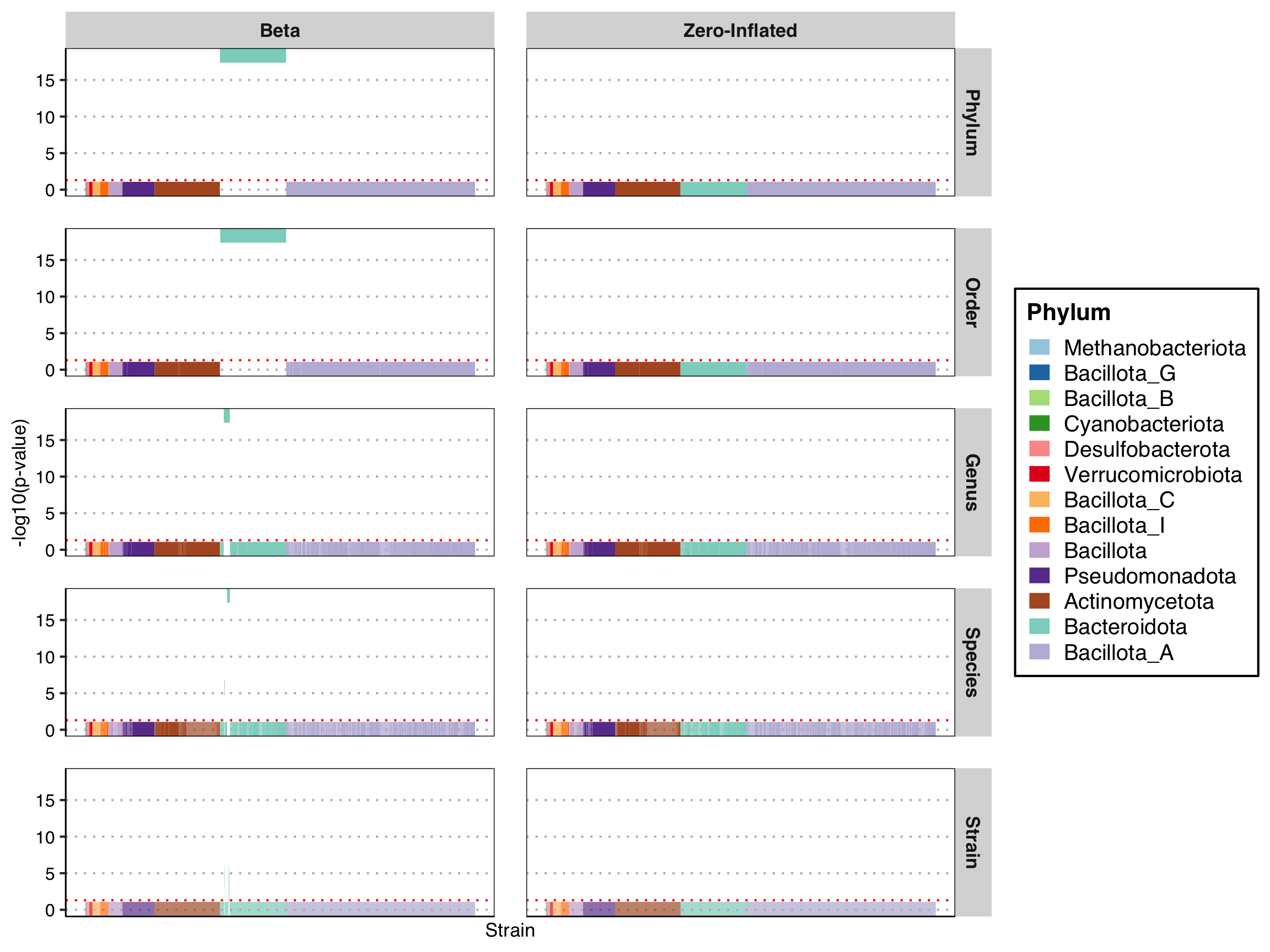
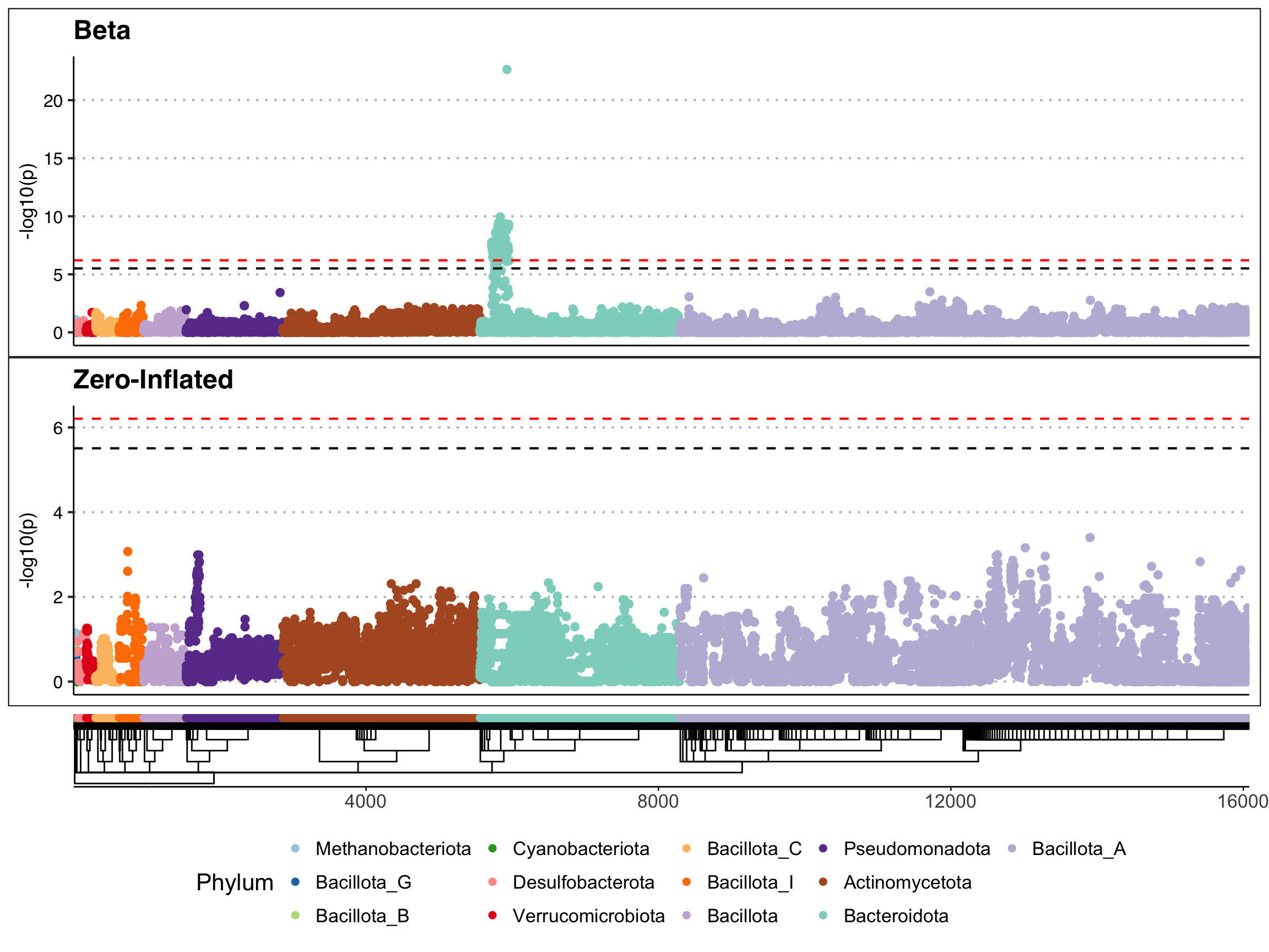
# All 76 hits from the same species
table(th_c1$Species)


  Parabacteroides distasonis Parabacteroides distasonis_A 
                          55                           21

Show code

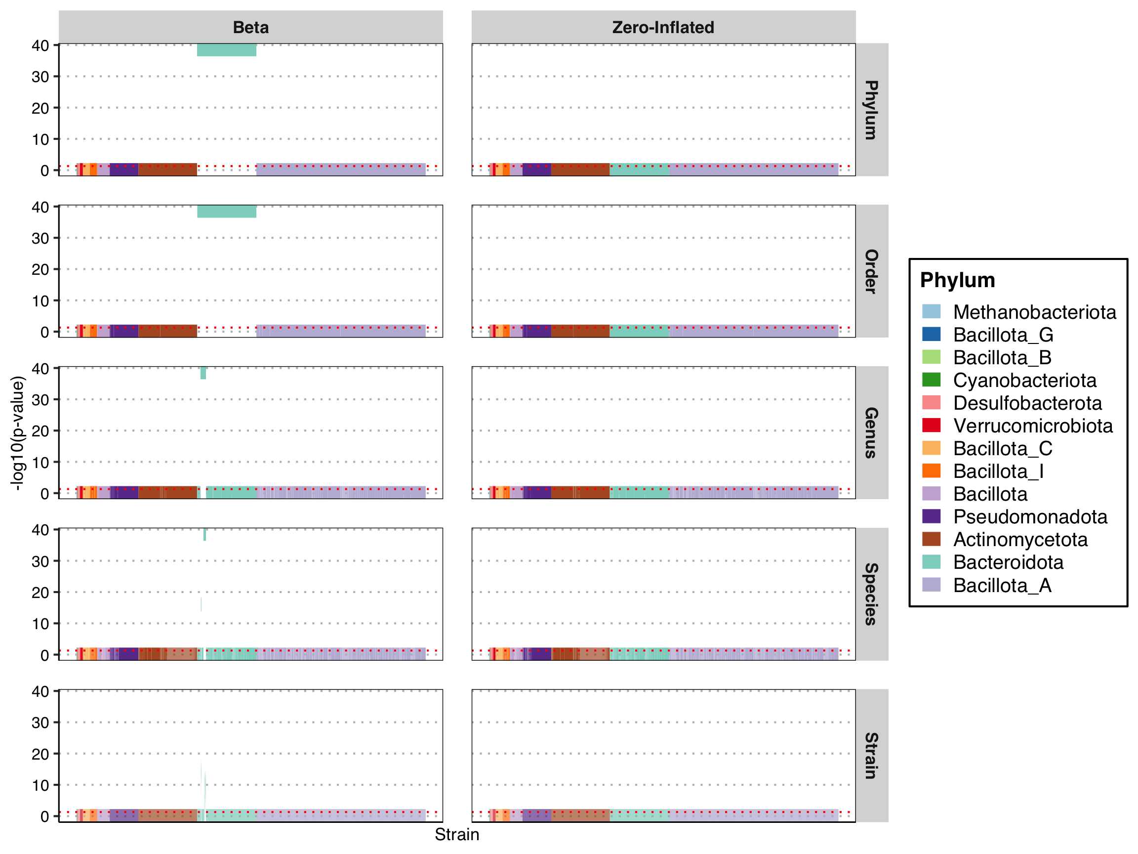
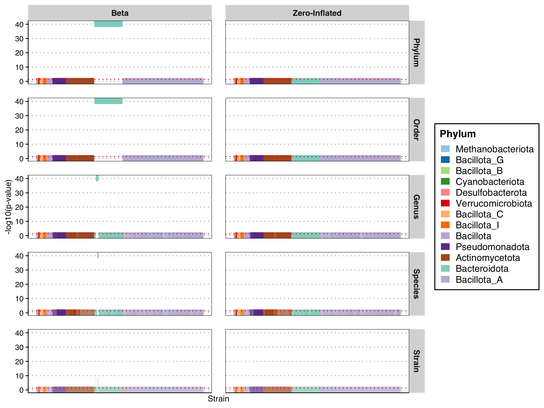
plot_manhattan(fit_zib_99_c1, taxonomy = tax_99, method = "BH", tax_levels = c("Order", "Phylum", "Genus", "Species"))

! # Invaild edge matrix for <phylo>. A <tbl_df> is returned.
! # Invaild edge matrix for <phylo>. A <tbl_df> is returned.
! # Invaild edge matrix for <phylo>. A <tbl_df> is returned.
! # Invaild edge matrix for <phylo>. A <tbl_df> is returned.

Warning: Using `size` aesthetic for lines was deprecated in ggplot2 3.4.0.
ℹ Please use `linewidth` instead.
ℹ The deprecated feature was likely used in the strainspy package.
  Please report the issue at <https://github.com/gtonkinhill/strainspy/issues>.

Show code

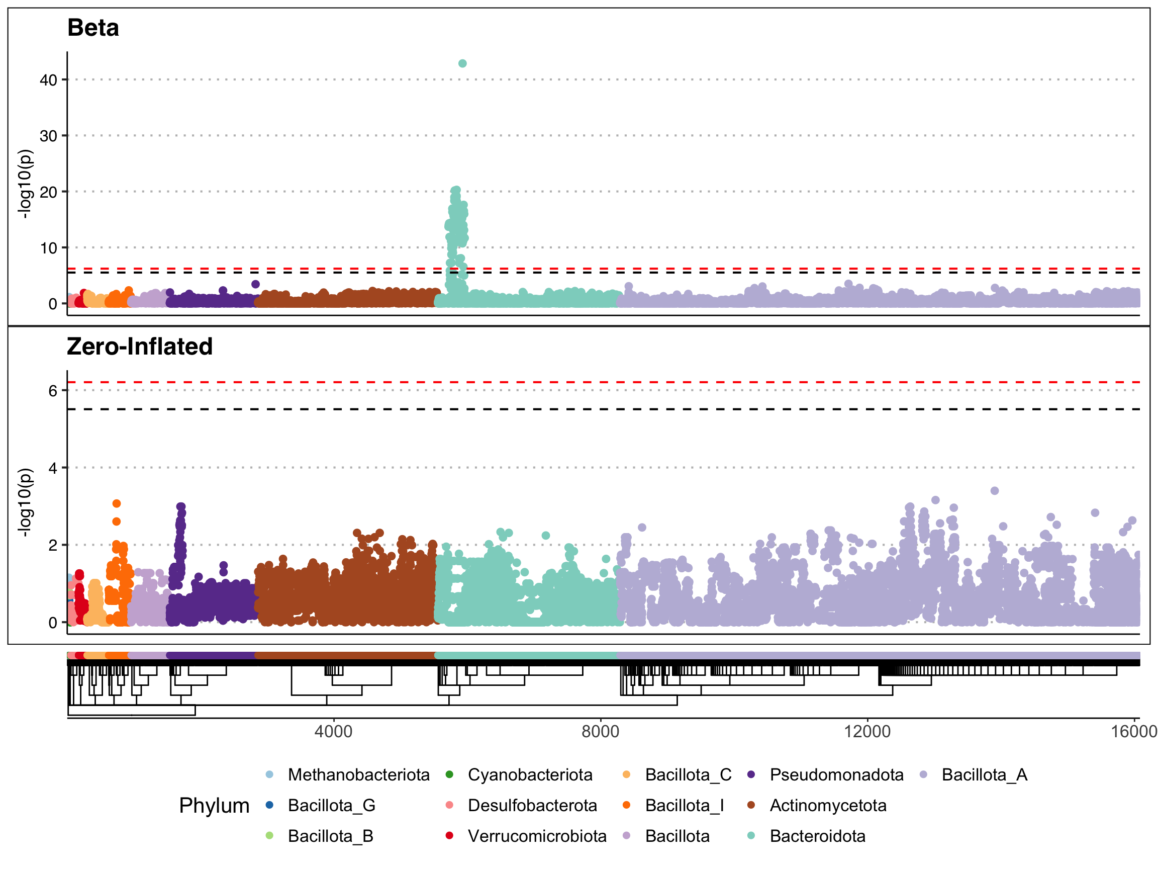
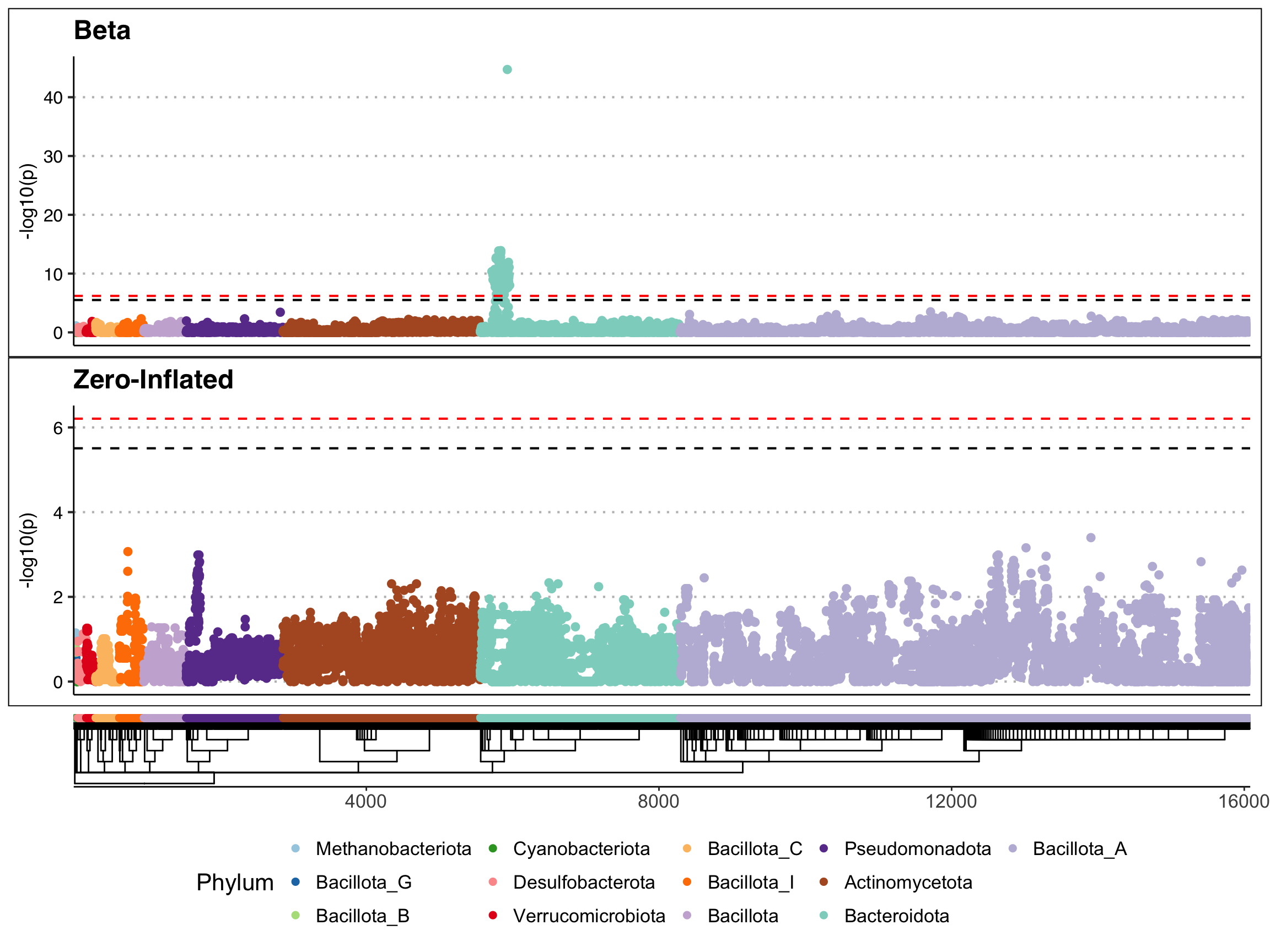
plot_manhattan(fit_zib_99_c1, taxonomy = tax_99, aggregate_by_taxa = F)

! # Invaild edge matrix for <phylo>. A <tbl_df> is returned.
! # Invaild edge matrix for <phylo>. A <tbl_df> is returned.
! # Invaild edge matrix for <phylo>. A <tbl_df> is returned.
! # Invaild edge matrix for <phylo>. A <tbl_df> is returned.
! # Invaild edge matrix for <phylo>. A <tbl_df> is returned.
! # Invaild edge matrix for <phylo>. A <tbl_df> is returned.

Show code

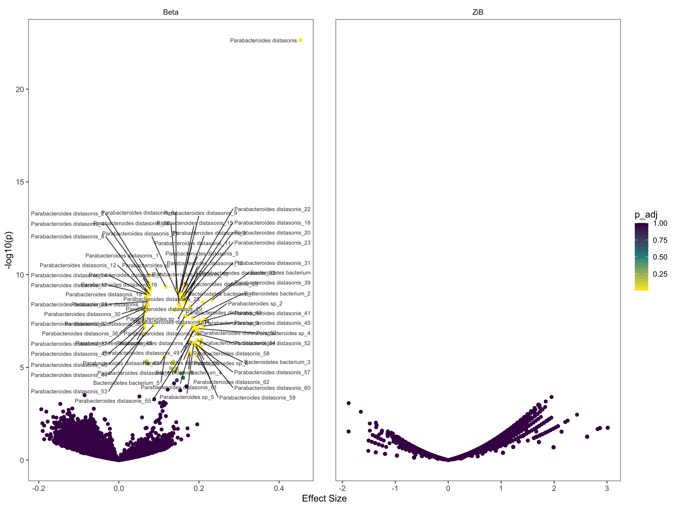
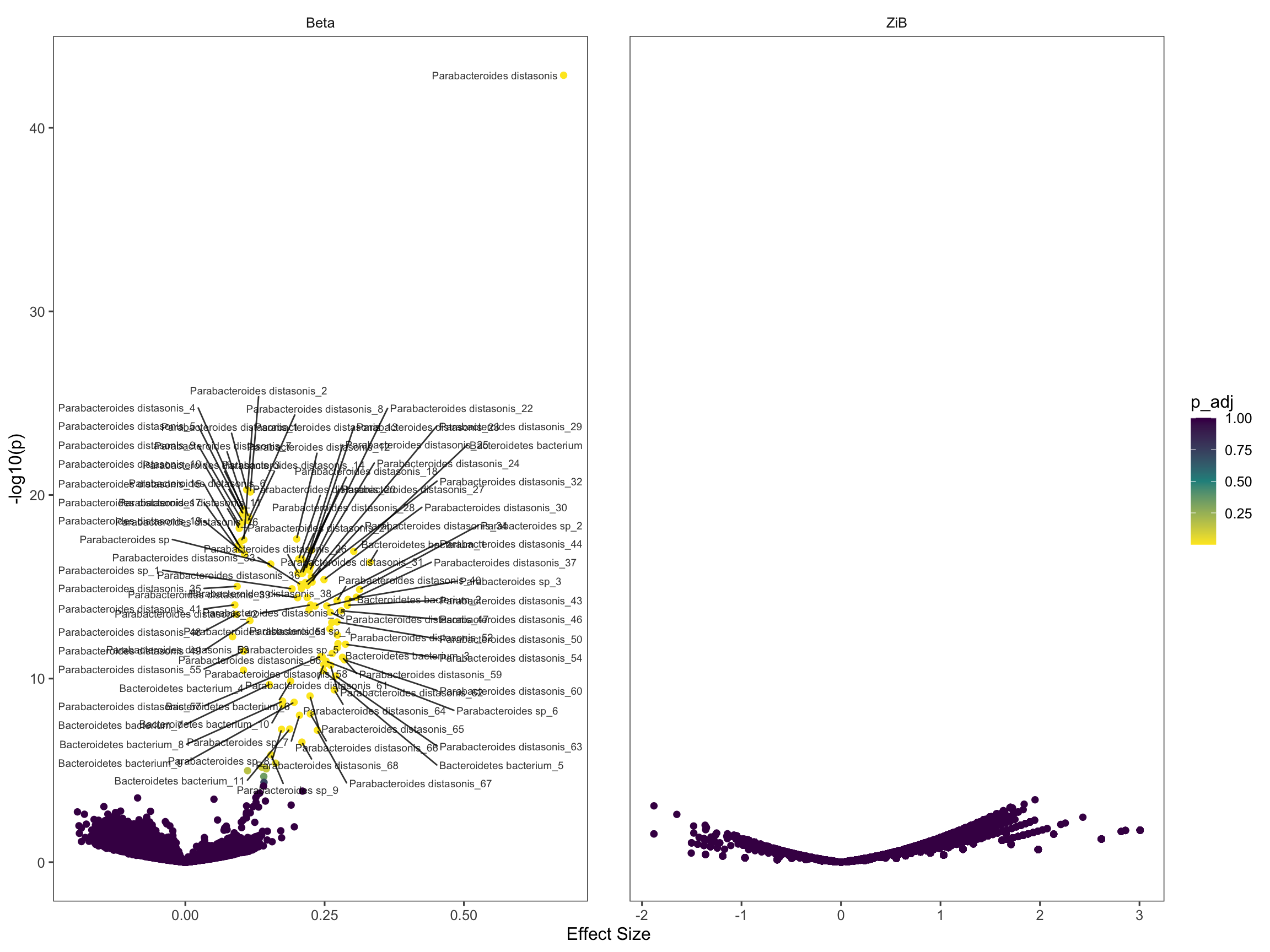
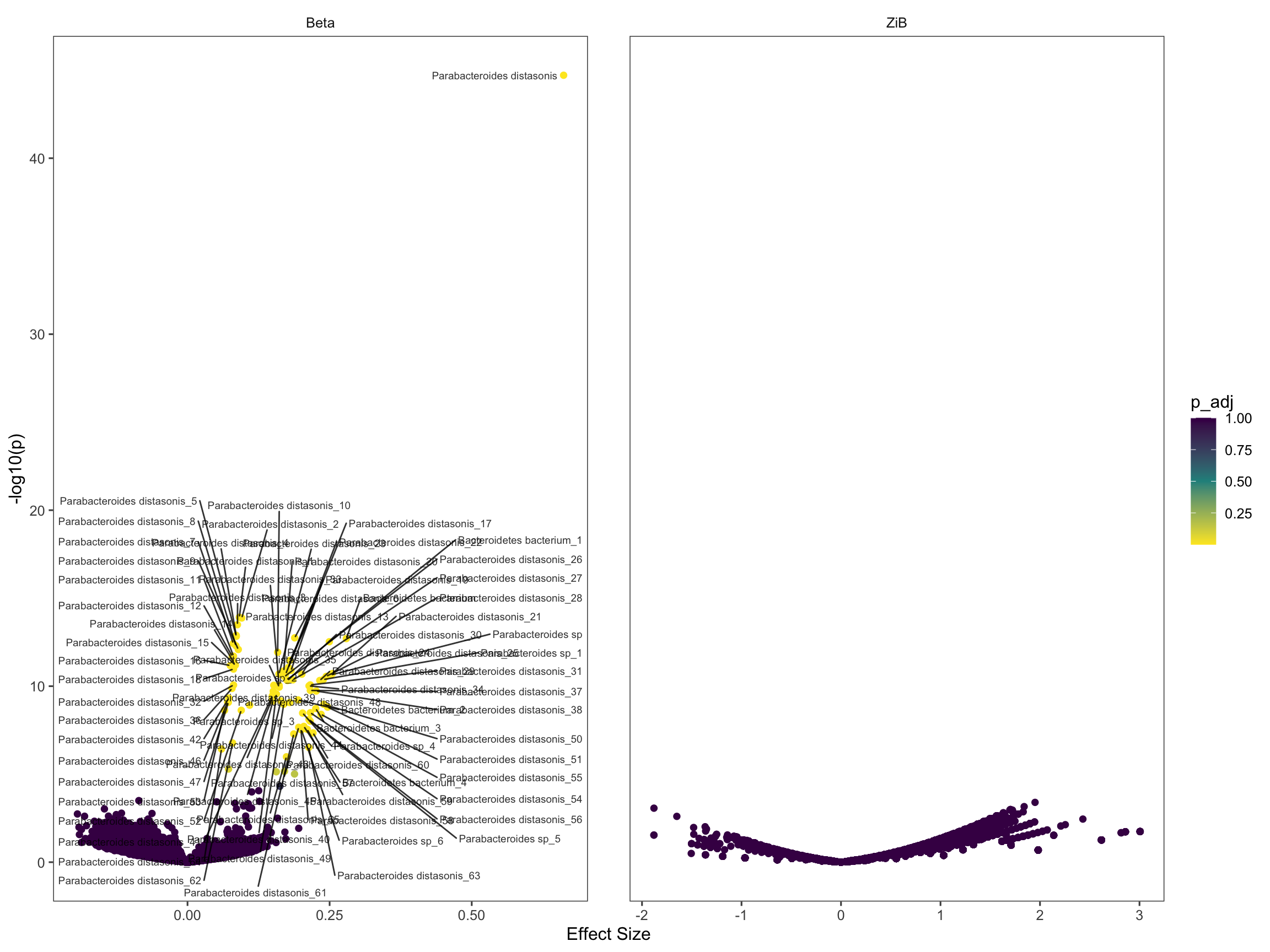
plot_volcano(fit_zib_99_c1, label = T)

Found 16081 tophits for spikedTRUE at alpha = 1 using holm

Show code

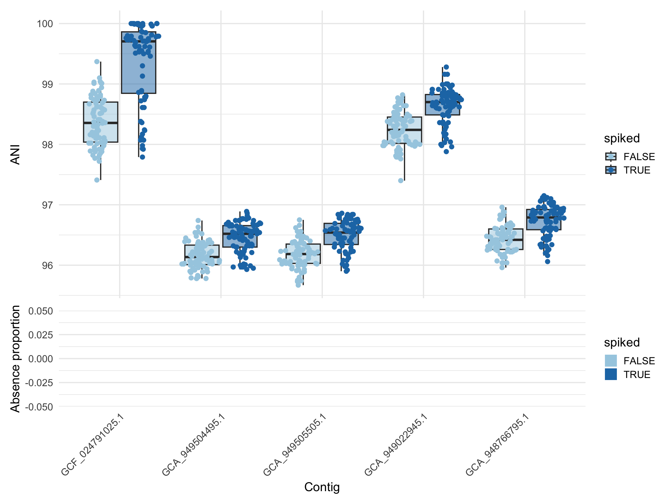
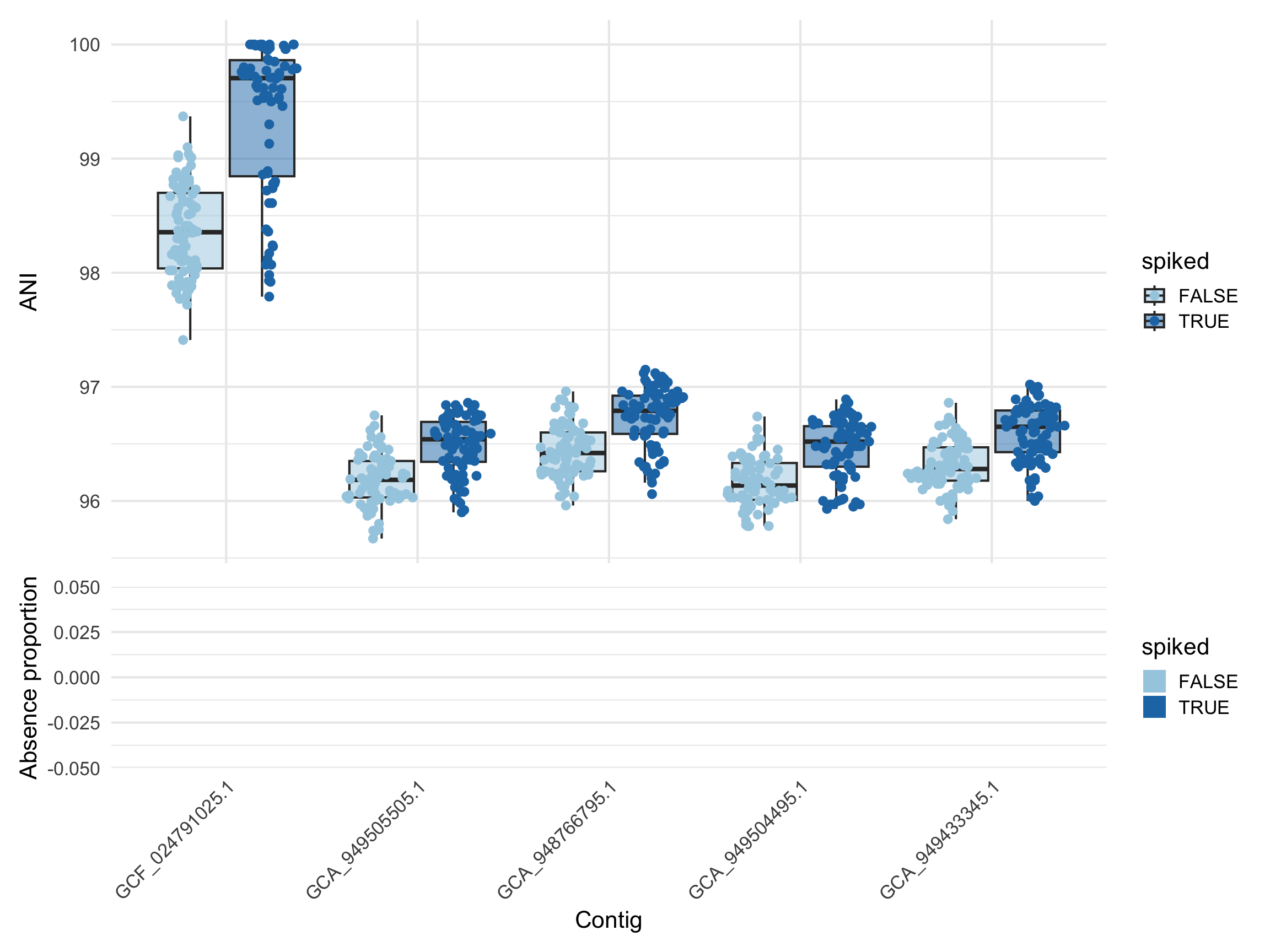
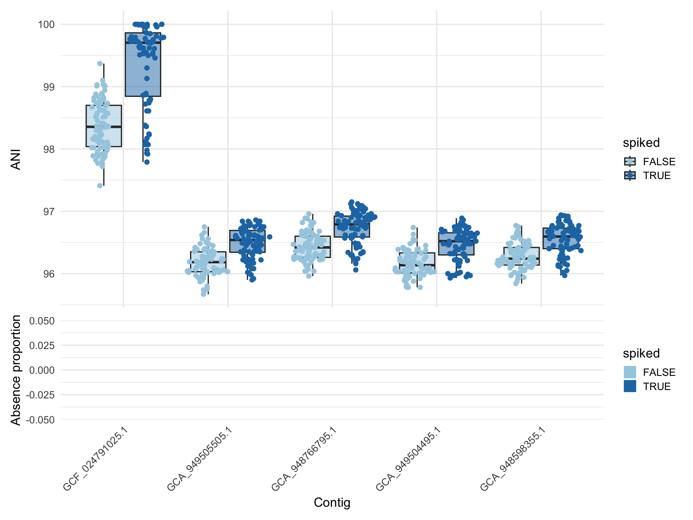
plot_ani_dist(d_q99, phenotype = 'spiked', contigs = th_c1$Contig_name[1:5], contig_names = th_c1$Genome_file[1:5])

Show code

# Parabacteroides distasonis is in all samples, so, this can only be a beta hit!
# GCF_024791025.1 is the top hit - it is the spiked strain. And for the spiked samples, the ANI is 100%

query 99, cov3x

Show code

# baseline false samples and higher coverage ones
rm_idx = c(sapply(ss, function(x) which(colnames(d_q99) %in% x)), grep("_sx1", colnames(d_q99)), grep("_sx5", colnames(d_q99)))
d_q99_test = d_q99[,-rm_idx]
dim(d_q99_test)

[1] 16081   100

Show code

# These 20 are spiked ata coverage of 3x
table(d_q99_test@colData$spiked)


FALSE  TRUE 
   80    20

Show code

save_path = "output_rds/spike_pdis_zib_q_99_cov3x.rds"
if(file.exists(save_path)){
  fit_zib_99_c3 <- readRDS(save_path)
} else {
  system.time({
    ebp = compute_eb_priors(d_q99_test, design, nthreads = parallel::detectCores())
    fit_zib_99_c3 <- glmZiBFit(d_q99_test, design, nthreads = parallel::detectCores(), MAP_prior = ebp)
  })
  saveRDS(fit_zib_99_c3, save_path)
}

th_c3 = strainspy:::add_tax2tophits(top_hits(fit_zib_99_c3), tax_99)

Found 91 tophits for spikedTRUE at alpha = 0.05 using holm

Show code

# All 91 hits from the same species
table(th_c3$Species)


  Parabacteroides distasonis Parabacteroides distasonis_A 
                          70                           21

Show code

plot_manhattan(fit_zib_99_c3, taxonomy = tax_99, method = "BH", tax_levels = c("Order", "Phylum", "Genus", "Species"))

! # Invaild edge matrix for <phylo>. A <tbl_df> is returned.
! # Invaild edge matrix for <phylo>. A <tbl_df> is returned.
! # Invaild edge matrix for <phylo>. A <tbl_df> is returned.
! # Invaild edge matrix for <phylo>. A <tbl_df> is returned.

Show code

plot_manhattan(fit_zib_99_c3, taxonomy = tax_99, aggregate_by_taxa = F)

! # Invaild edge matrix for <phylo>. A <tbl_df> is returned.
! # Invaild edge matrix for <phylo>. A <tbl_df> is returned.
! # Invaild edge matrix for <phylo>. A <tbl_df> is returned.
! # Invaild edge matrix for <phylo>. A <tbl_df> is returned.
! # Invaild edge matrix for <phylo>. A <tbl_df> is returned.
! # Invaild edge matrix for <phylo>. A <tbl_df> is returned.

Show code

plot_volcano(fit_zib_99_c3, label = T)

Found 16081 tophits for spikedTRUE at alpha = 1 using holm

Show code

plot_ani_dist(d_q99, phenotype = 'spiked', contigs = th_c3$Contig_name[1:5], contig_names = th_c3$Genome_file[1:5])

Show code

# Parabacteroides distasonis is in all samples, so, this can only be a beta hit!
# GCF_024791025.1 is the top hit - it is the spiked strain. And for the spiked samples, the ANI is 100%

query 99, cov5x

Show code

# baseline false samples and higher coverage ones
rm_idx = c(sapply(ss, function(x) which(colnames(d_q99) %in% x)), grep("_sx1", colnames(d_q99)), grep("_sx3", colnames(d_q99)))
d_q99_test = d_q99[,-rm_idx]
dim(d_q99_test)

[1] 16081   100

Show code

# These 20 are spiked ata coverage of 3x
table(d_q99_test@colData$spiked)


FALSE  TRUE 
   80    20

Show code

save_path = "output_rds/spike_pdis_zib_q_99_cov5x.rds"
if(file.exists(save_path)){
  fit_zib_99_c5 <- readRDS(save_path)
} else {
  system.time({
    ebp = compute_eb_priors(d_q99_test, design, nthreads = parallel::detectCores())
    fit_zib_99_c5 <- glmZiBFit(d_q99_test, design, nthreads = parallel::detectCores(), MAP_prior = ebp)
  })
  saveRDS(fit_zib_99_c5, save_path)
}

th_c5 = strainspy:::add_tax2tophits(top_hits(fit_zib_99_c5), tax_99)

Found 78 tophits for spikedTRUE at alpha = 0.05 using holm

Show code

# All 91 hits from the same species
table(th_c5$Species)


  Parabacteroides distasonis Parabacteroides distasonis_A 
                          57                           21

Show code

plot_manhattan(fit_zib_99_c5, taxonomy = tax_99, method = "BH", tax_levels = c("Order", "Phylum", "Genus", "Species"))

! # Invaild edge matrix for <phylo>. A <tbl_df> is returned.
! # Invaild edge matrix for <phylo>. A <tbl_df> is returned.
! # Invaild edge matrix for <phylo>. A <tbl_df> is returned.
! # Invaild edge matrix for <phylo>. A <tbl_df> is returned.

Show code

plot_manhattan(fit_zib_99_c5, taxonomy = tax_99, aggregate_by_taxa = F)

! # Invaild edge matrix for <phylo>. A <tbl_df> is returned.
! # Invaild edge matrix for <phylo>. A <tbl_df> is returned.
! # Invaild edge matrix for <phylo>. A <tbl_df> is returned.
! # Invaild edge matrix for <phylo>. A <tbl_df> is returned.
! # Invaild edge matrix for <phylo>. A <tbl_df> is returned.
! # Invaild edge matrix for <phylo>. A <tbl_df> is returned.

Show code

plot_volcano(fit_zib_99_c5, label = T)

Found 16081 tophits for spikedTRUE at alpha = 1 using holm

Show code

plot_ani_dist(d_q99, phenotype = 'spiked', contigs = th_c5$Contig_name[1:5], contig_names = th_c5$Genome_file[1:5])

Show code

# Parabacteroides distasonis is in all samples, so, this can only be a beta hit!
# GCF_024791025.1 is the top hit - it is the spiked strain. And for the spiked samples, the ANI is 100%

StrainSpy works regardless of coverage, now to test AnPan

Load data and prepare for testing

Show code

library(anpan)

• This is anpan version 0.3.0
• Read the guide: run anpan::anpan_vignette()
• Get help: Visit the biobakery help forum at <https://forum.biobakery.org/>
• Parallelize: Run `future::plan()` as appropriate for your system.
• Activate progress bars: `library(progressr); handlers(global=TRUE)`

Show code

library(ape)


Attaching package: 'ape'

The following object is masked from 'package:dplyr':

    where

Show code

library(tibble)
tree = read.tree("p_distasonis_sims/spiked_tree.tre")

metadata = tibble(sample_id = tree$tip.label,
                  spiked   = as.factor(sapply(tree$tip.label, function(x) x%in% c(ss, sub("_", "_1_", paste(ss_spikes, ".fastq", sep = "")) ))) )

table(metadata$spiked)


FALSE  TRUE 
   64    72

Show code

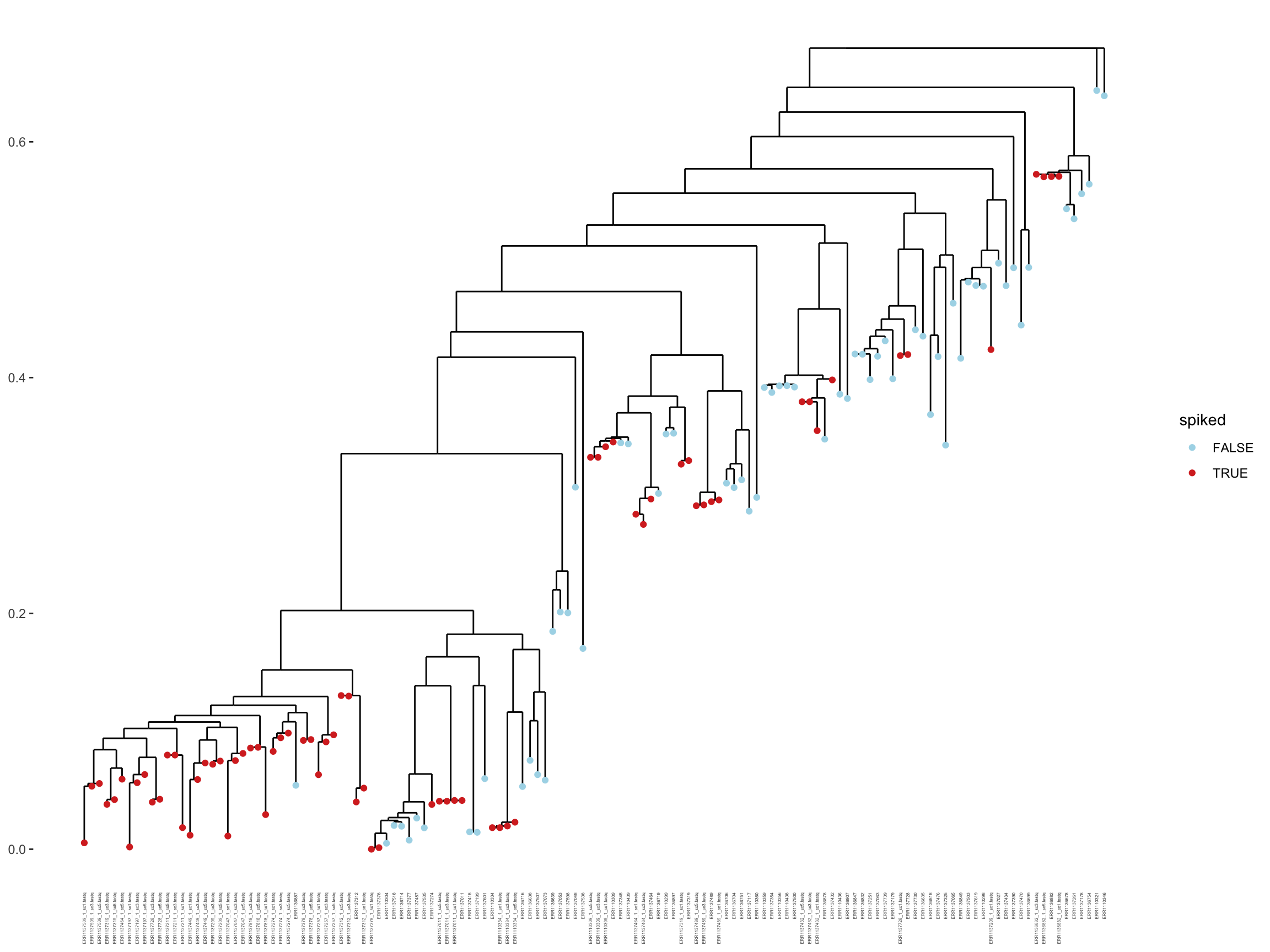
plot_outcome_tree(tree,
                  metadata, 
                  covariates = c(),
                  outcome    = "spiked")

Warning: `aes_string()` was deprecated in ggplot2 3.0.0.
ℹ Please use tidy evaluation idioms with `aes()`.
ℹ See also `vignette("ggplot2-in-packages")` for more information.
ℹ The deprecated feature was likely used in the anpan package.
  Please report the issue to the authors.

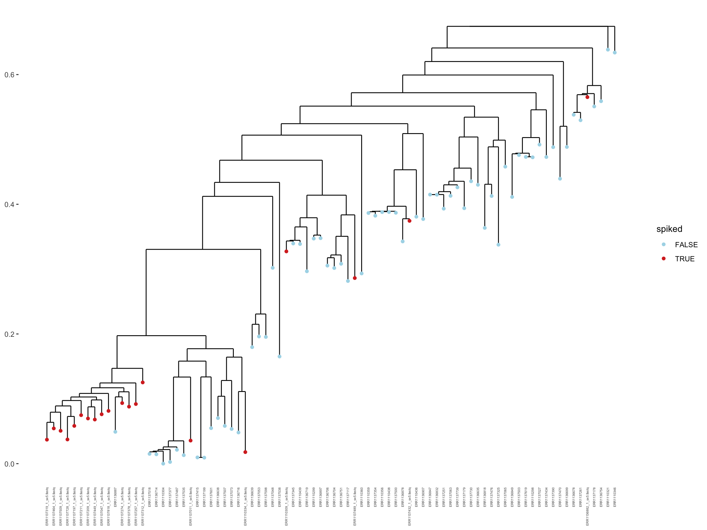
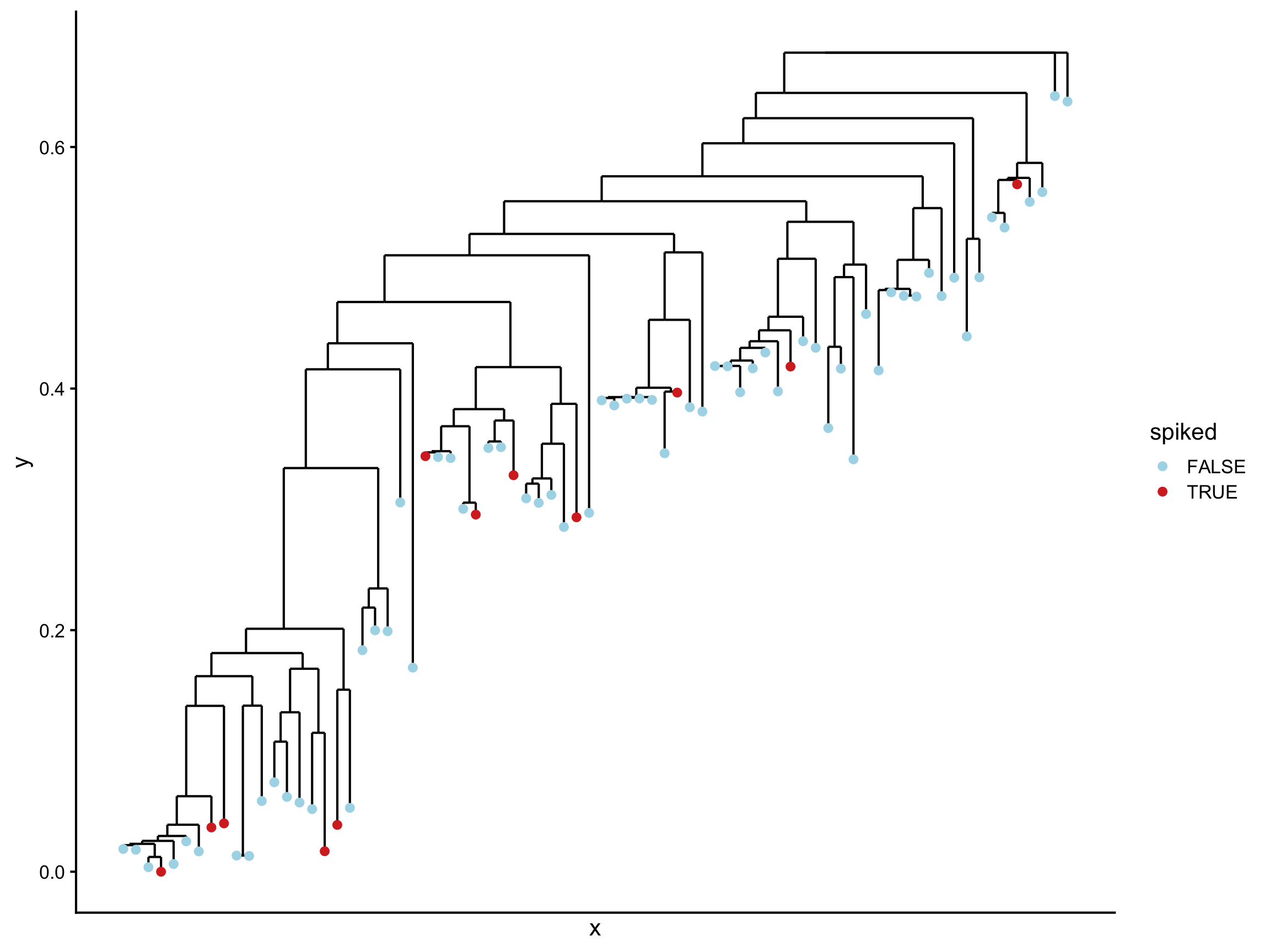
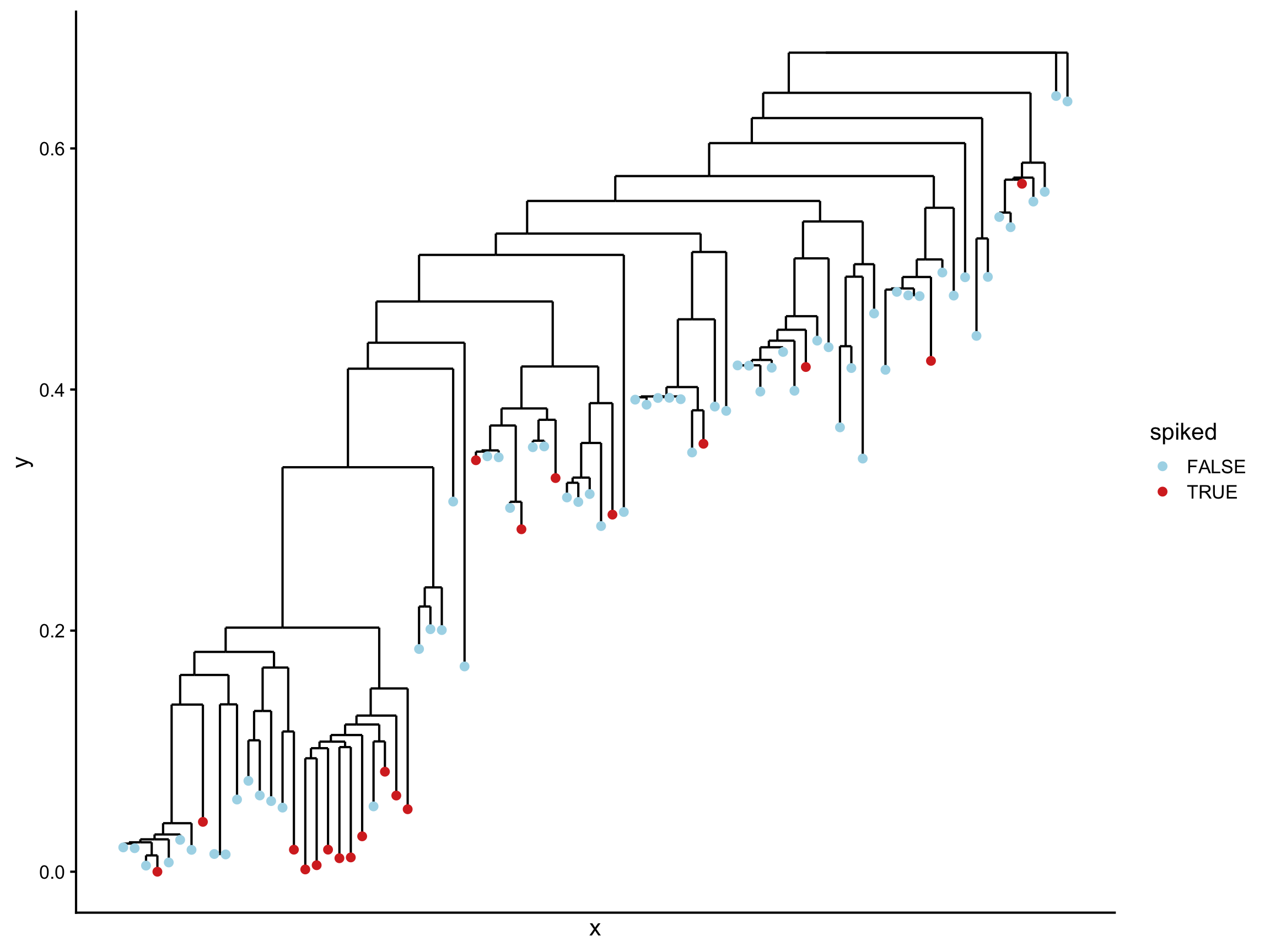
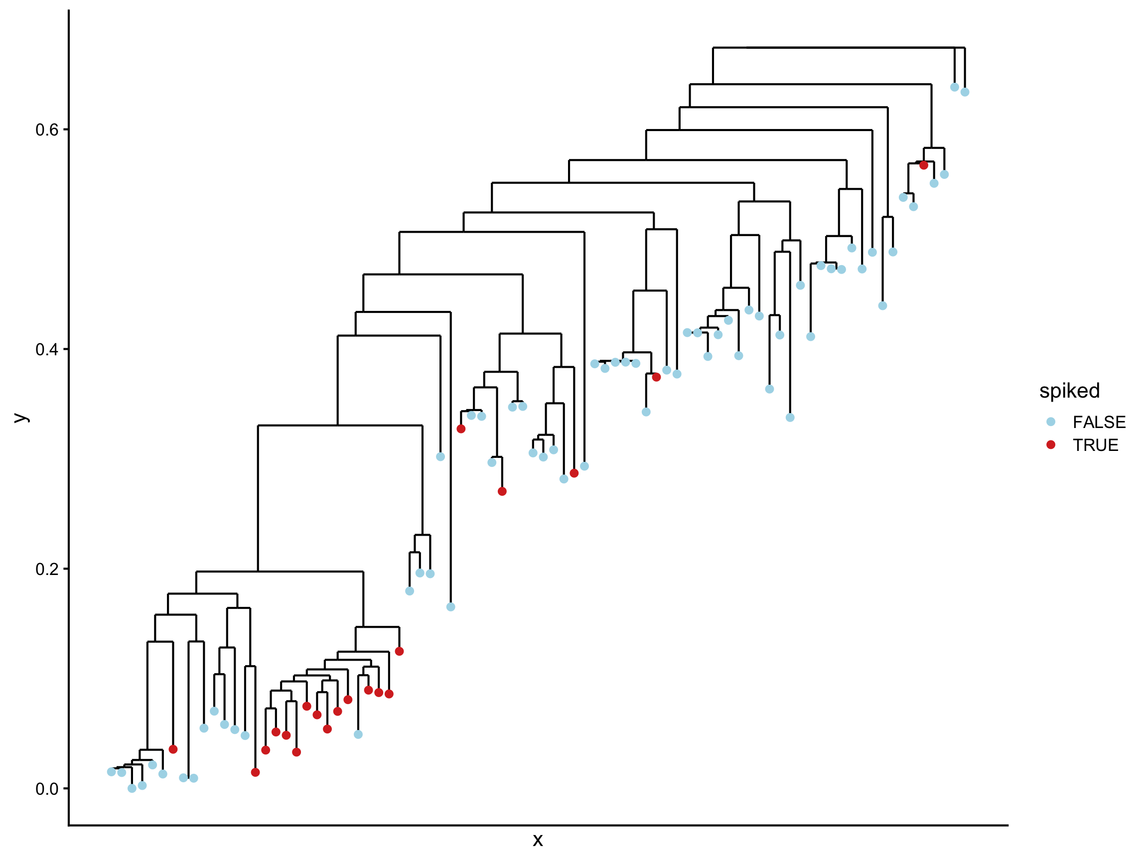
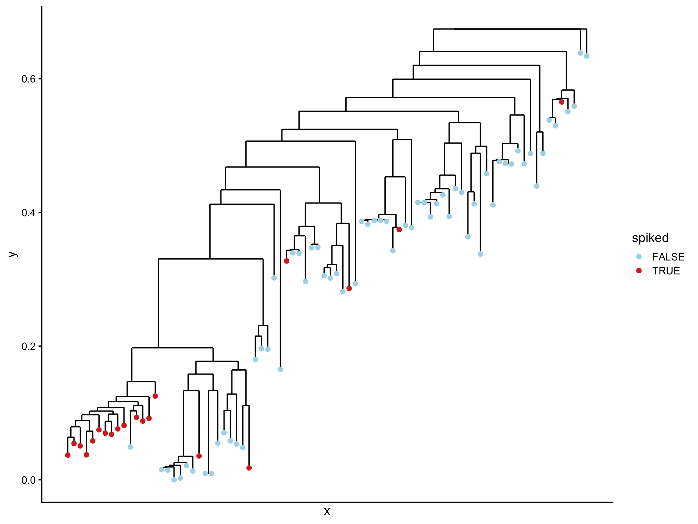
Looks like the left-most branch has a bunch of spiked ones, it’ll be interesting to see variation with coverage

anPan PGLMM

baseline (no signal)

Show code

# This simulation does not have any signal, we shouldn't detect anything!

# Subset
rm_idx = grep("_sx", metadata$sample_id)

metadata_test = metadata[-rm_idx, ]
table(metadata_test$spiked)


FALSE  TRUE 
   64    12

Show code

# Only 76/100 samples had P. dist at a detectable level for strainphlan
# These TRUE = 12 are NOT spiked in, this is just to show there is no detectable signal

# Drop the same leaves from the tree
tree_test = drop.tip(tree, metadata$sample_id[rm_idx])
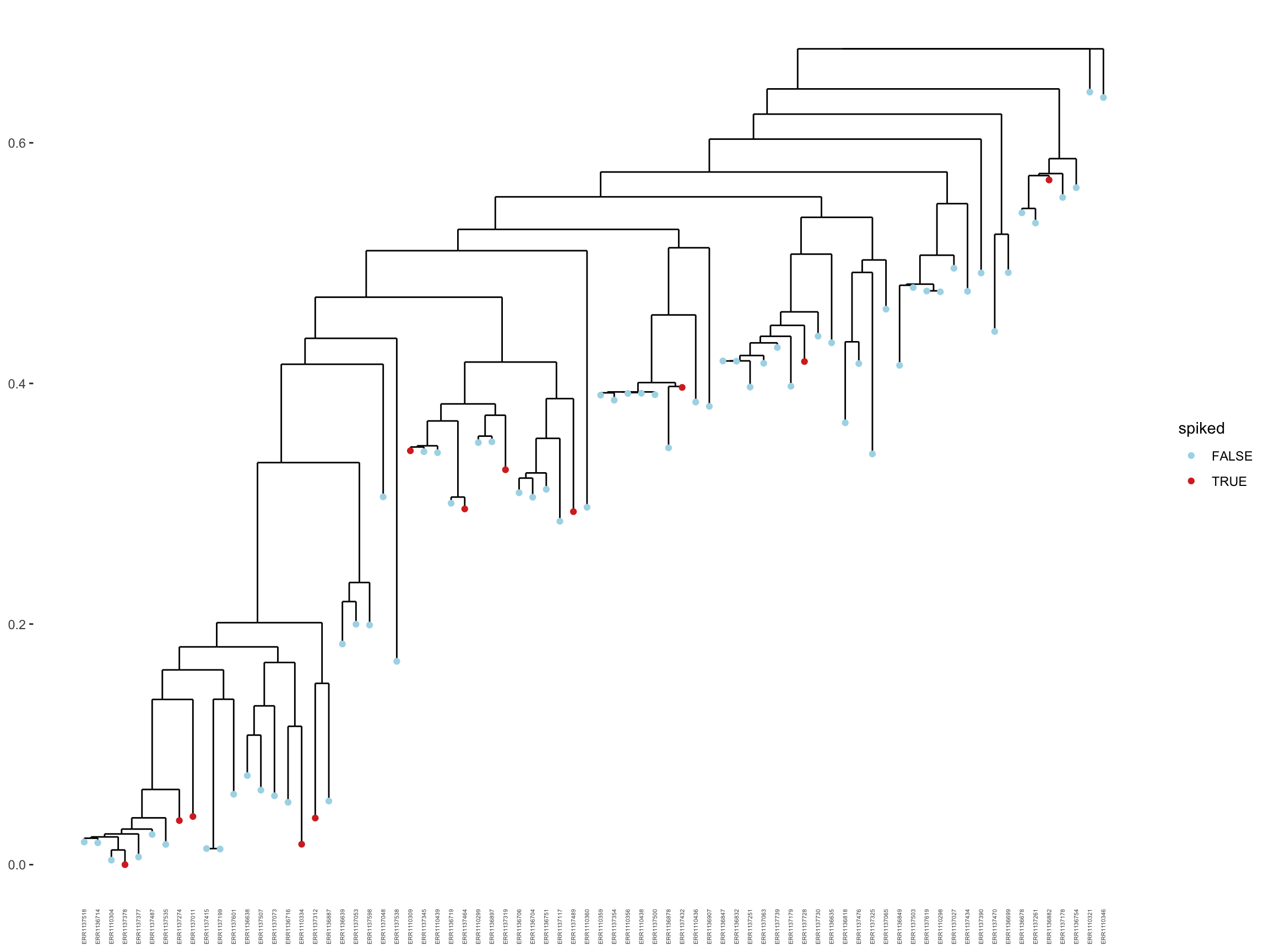
plot_outcome_tree(tree_test,
                  metadata_test, 
                  covariates = c(),
                  outcome    = "spiked")

Show code

# Clearly no signal

save_path = "output_rds/spike_pdis_anpan_bl.rds"
if(file.exists(save_path)){
  anpan_res_bl <- readRDS(save_path)
} else {
  system.time({
    anpan_res_bl = anpan_pglmm(meta_file       = metadata_test,
                               tree_file       = tree_test,
                               outcome         = "spiked",
                               family          = "binomial",
                               bug_name        = "Pdis",
                               reg_noise       = TRUE,
                               loo_comparison  = TRUE,
                               run_diagnostics = FALSE,
                               refresh         = 500,
                               show_plot_tree  = FALSE,
                               show_post       = FALSE)
  })
  saveRDS(anpan_res_bl, save_path)
}

anpan_res_bl$loo$comparison

            elpd_diff   se_diff  elpd_loo se_elpd_loo    p_loo  se_p_loo
base_fit   0.00000000 0.0000000 -34.10157    5.094281 0.855544 0.1756572
pglmm_fit -0.09731679 0.1441665 -34.19889    5.065588 1.205773 0.2441358
             looic se_looic
base_fit  68.20314 10.18856
pglmm_fit 68.39777 10.13118
attr(,"class")
[1] "compare.loo" "matrix"      "array"

Clearly no signal - confirmed by PGLMM

cov1x

Show code

# Subset
rm_idx = unlist(c(sapply(ss, function(x) which(metadata$sample_id %in% x)), grep("_sx3", metadata$sample_id), grep("_sx5", metadata$sample_id)))

metadata_test = metadata[-rm_idx, ]
table(metadata_test$spiked)


FALSE  TRUE 
   64    20

Show code

# Only 20/20 spiked samples are now detected, but only non spiked are present - should be plenty 

# Drop the same leaves from the tree
tree_test = drop.tip(tree, metadata$sample_id[rm_idx])
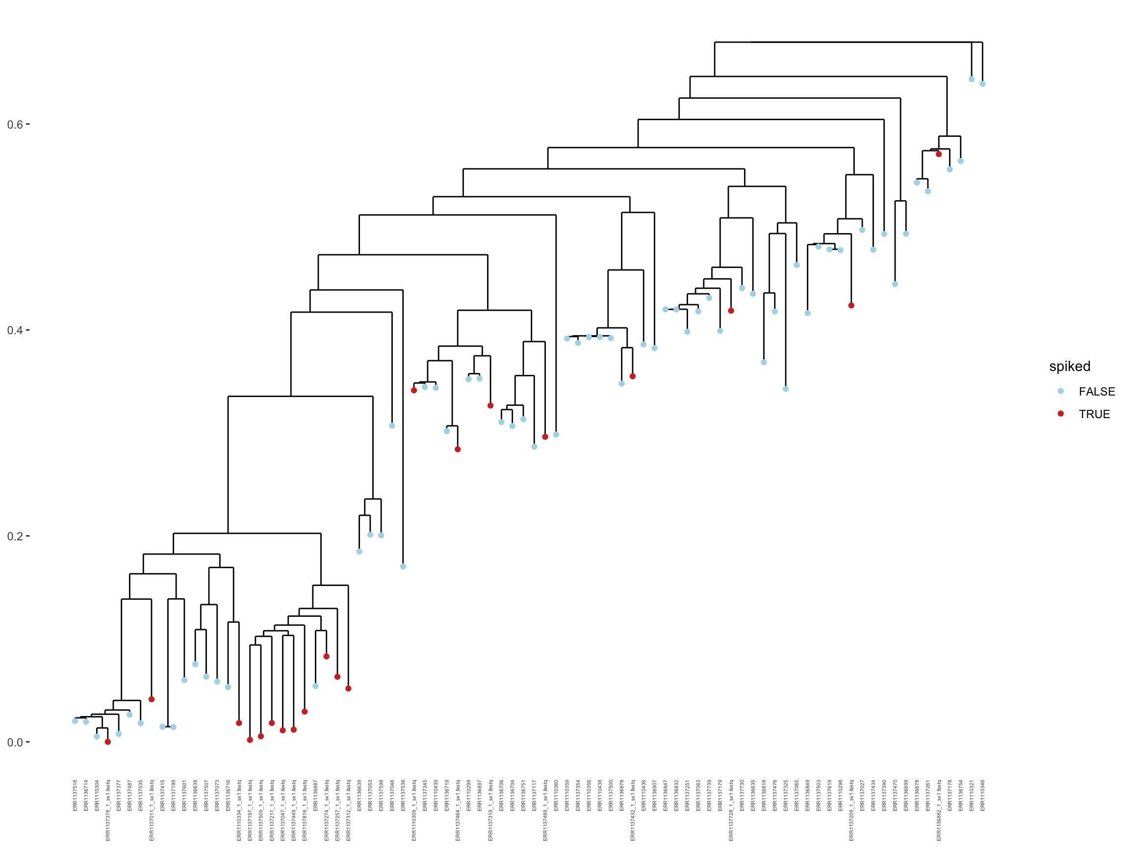
plot_outcome_tree(tree_test,
                  metadata_test, 
                  covariates = c(),
                  outcome    = "spiked")

Show code

# Signal is a bit weak

save_path = "output_rds/spike_pdis_anpan_cov1x.rds"
if(file.exists(save_path)){
  anpan_res_c1 <- readRDS(save_path)
} else {
  system.time({
    anpan_res_c1 = anpan_pglmm(meta_file       = metadata_test,
                               tree_file       = tree_test,
                               outcome         = "spiked",
                               family          = "binomial",
                               bug_name        = "Pdis",
                               reg_noise       = TRUE,
                               loo_comparison  = TRUE,
                               run_diagnostics = FALSE,
                               refresh         = 500,
                               show_plot_tree  = FALSE,
                               show_post       = FALSE)
  })
  saveRDS(anpan_res_c1, save_path)
}

anpan_res_c1$loo$comparison

          elpd_diff   se_diff  elpd_loo se_elpd_loo     p_loo  se_p_loo
pglmm_fit  0.000000 0.0000000 -45.52922    4.278753 2.1446260 0.2959159
base_fit  -1.612409 0.8160137 -47.14163    4.425549 0.9993287 0.1292906
             looic se_looic
pglmm_fit 91.05844 8.557506
base_fit  94.28326 8.851099
attr(,"class")
[1] "compare.loo" "matrix"      "array"

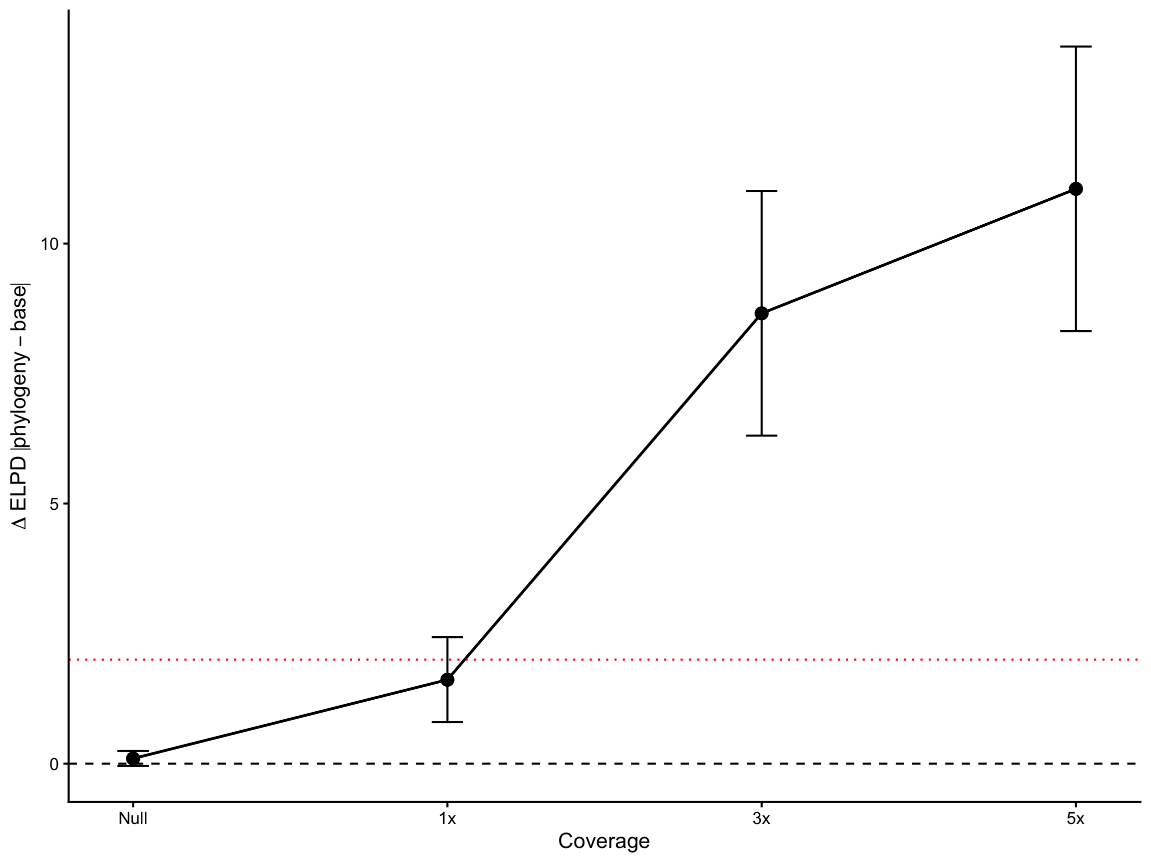
The phylogenetic model seems to fit better, but the difference doesn’t seem clear (less than 2 standard errors difference in ELPD).

cov3x

Show code

# Subset
rm_idx = unlist(c(sapply(ss, function(x) which(metadata$sample_id %in% x)), grep("_sx1", metadata$sample_id), grep("_sx5", metadata$sample_id)))

metadata_test = metadata[-rm_idx, ]
table(metadata_test$spiked)


FALSE  TRUE 
   64    20

Show code

# Only 20/20 spiked samples are now detected, but only non spiked are present - should be plenty 

# Drop the same leaves from the tree
tree_test = drop.tip(tree, metadata$sample_id[rm_idx])
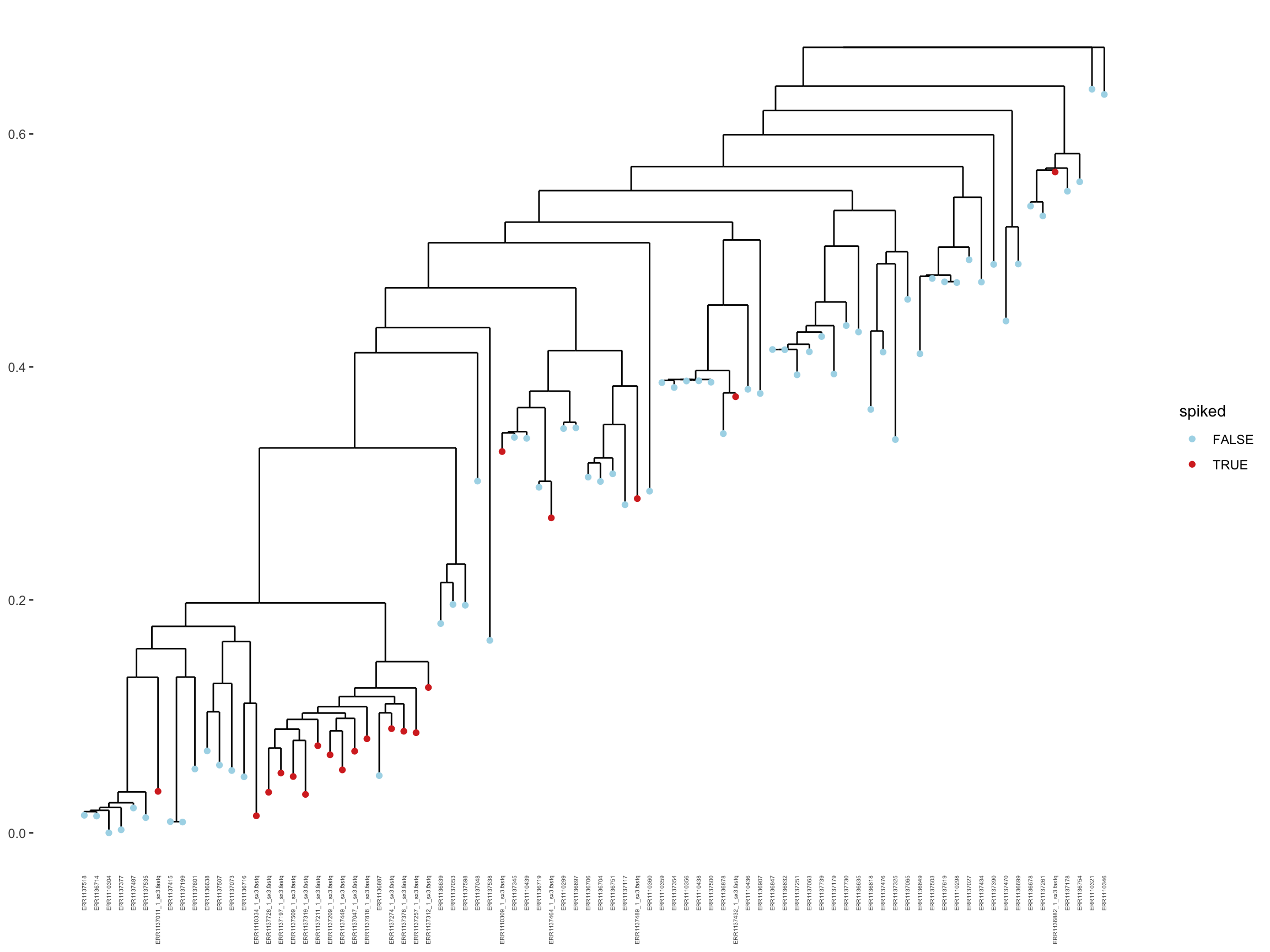
plot_outcome_tree(tree_test,
                  metadata_test, 
                  covariates = c(),
                  outcome    = "spiked")

Show code

# Clearly signal is present

save_path = "output_rds/spike_pdis_anpan_cov3x.rds"
if(file.exists(save_path)){
  anpan_res_c3 <- readRDS(save_path)
} else {
  system.time({
    anpan_res_c3 = anpan_pglmm(meta_file       = metadata_test,
                               tree_file       = tree_test,
                               outcome         = "spiked",
                               family          = "binomial",
                               bug_name        = "Pdis",
                               reg_noise       = TRUE,
                               loo_comparison  = TRUE,
                               run_diagnostics = FALSE,
                               refresh         = 500,
                               show_plot_tree  = FALSE,
                               show_post       = FALSE)
  })
  saveRDS(anpan_res_c3, save_path)
}

anpan_res_c3$loo$comparison

          elpd_diff  se_diff  elpd_loo se_elpd_loo    p_loo  se_p_loo    looic
pglmm_fit  0.000000 0.000000 -38.39092    3.918328 2.993786 0.4993756 76.78183
base_fit  -8.657758 2.351852 -47.04867    4.399150 0.902703 0.1160073 94.09735
          se_looic
pglmm_fit 7.836656
base_fit  8.798300
attr(,"class")
[1] "compare.loo" "matrix"      "array"

The phylogenetic model seems to fit better, and the difference seems clear (more than 2 standard errors difference in ELPD).

cov5x

Show code

# Subset
rm_idx = unlist(c(sapply(ss, function(x) which(metadata$sample_id %in% x)), grep("_sx1", metadata$sample_id), grep("_sx3", metadata$sample_id)))

metadata_test = metadata[-rm_idx, ]
table(metadata_test$spiked)


FALSE  TRUE 
   64    20

Show code

# Only 20/20 spiked samples are now detected, but only non spiked are present - should be plenty 

# Drop the same leaves from the tree
tree_test = drop.tip(tree, metadata$sample_id[rm_idx])
plot_outcome_tree(tree_test,
                  metadata_test, 
                  covariates = c(),
                  outcome    = "spiked")

Show code

# Clearly dominant signal

save_path = "output_rds/spike_pdis_anpan_cov5x.rds"
if(file.exists(save_path)){
  anpan_res_c5 <- readRDS(save_path)
} else {
  system.time({
    anpan_res_c5 = anpan_pglmm(meta_file       = metadata_test,
                               tree_file       = tree_test,
                               outcome         = "spiked",
                               family          = "binomial",
                               bug_name        = "Pdis",
                               reg_noise       = TRUE,
                               loo_comparison  = TRUE,
                               run_diagnostics = FALSE,
                               refresh         = 500,
                               show_plot_tree  = FALSE,
                               show_post       = FALSE)
  })
  saveRDS(anpan_res_c5, save_path)
}

anpan_res_c5$loo$comparison

          elpd_diff  se_diff  elpd_loo se_elpd_loo    p_loo  se_p_loo    looic
pglmm_fit   0.00000 0.000000 -36.09019    3.860277 2.839414 0.5063496 72.18038
base_fit  -11.05142 2.735972 -47.14161    4.429170 1.000522 0.1284311 94.28322
          se_looic
pglmm_fit 7.720554
base_fit  8.858339
attr(,"class")
[1] "compare.loo" "matrix"      "array"

The phylogenetic model seems to fit better, and the difference seems clear (more than 2 standard errors difference in ELPD).

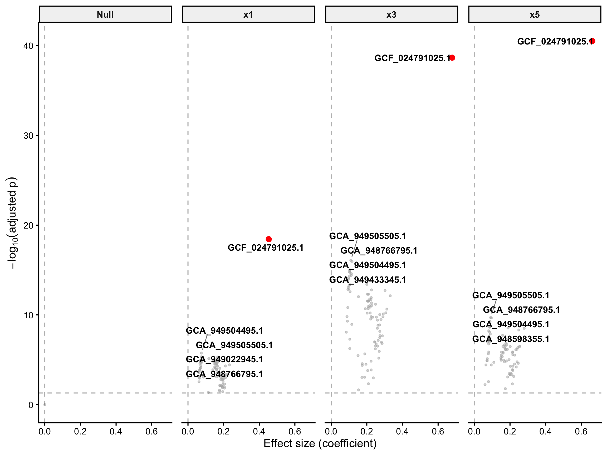
AnPan works as well - when there is signal in the phylogeny, it can detect it accurately. However, building the tree can be tricky if the strain coverage is low. StrainSpy can work equally well in the lower coverage simulations as well, without requiring a phylogeny.

Figure for paper

Show code

# strainspy result

spike = "GCF_024791025.1"

th_plt = rbind(cbind(th_c1, coverage = "x1"),
               cbind(th_c3, coverage = "x3"),
               cbind(th_c5, coverage =  "x5"))

th_plt[nrow(th_plt)+1, ] = th_plt[nrow(th_plt),]
# manually add the baseline hits (there are none!)
th_plt$coefficient[nrow(th_plt)] = 0 
th_plt$p_adjust[nrow(th_plt)] = 1
th_plt$coverage[nrow(th_plt)] = "Null"
th_plt$Contig_name[nrow(th_plt)] = ""


th_plt$neglog_p = -log10(th_plt$p_adjust)

label_df <- th_plt %>%
  group_by(coverage) %>%
  arrange(p_adjust, .by_group = TRUE) %>%
  slice_head(n = 5) %>%
  ungroup()

# No label needed for the fake point
rmidx = which(label_df$coverage == "Null")
if(length(rmidx) > 0) label_df = label_df[-rmidx, ]

top1 <- th_plt %>%
  group_by(coverage) %>%
  arrange(p_adjust) %>%
  slice(1)

ggplot(th_plt, aes(x = coefficient, y = neglog_p)) +
  geom_point(
    data = subset(th_plt, Genome_file != spike),
    aes(color = "other"),
    size = 1,
    alpha = 0.5
  ) +
  geom_point(
    data = subset(th_plt, Genome_file == spike),
    color = "red",
    size = 2.5,
    stroke = 1.2
  ) +
  geom_text_repel(
    data = label_df,
    aes(label = Genome_file),
    size = 4.5,
    fontface = "bold",
    box.padding = 0.4,
    point.padding = 0.3,
    segment.color = "grey50",
    max.overlaps = Inf
  ) + 
  
  scale_color_manual(values = c("grey70", "red")) +
  facet_wrap(~coverage, nrow = 1) +
  theme_classic() +
  labs(
    x = "Effect size (coefficient)",
    y = expression(-log[10](adjusted~p))
  ) +
  guides(color = "none") + 
  geom_vline(xintercept = 0, linetype = "dashed", alpha = 0.3) +
  geom_hline(yintercept = -log10(0.05), linetype = "dashed", alpha = 0.3) +
  theme_classic(base_size = 16) +
  theme(
    strip.background = element_rect(fill = "grey95"),
    strip.text = element_text(face = "bold"),
    panel.spacing = unit(1, "lines")
  )

Show code

# anpan result

## Null model
rm_idx = rm_idx = grep("_sx", metadata$sample_id)
metadata_test = metadata[-rm_idx, ]

# Drop the same leaves from the tree
tree_test = drop.tip(tree, metadata$sample_id[rm_idx])
tp_null = plot_outcome_tree(tree_test,
                        metadata_test, 
                        covariates = c(),
                        outcome    = "spiked", return_tree_df = T)

tp_null$tree_plot + theme_classic(base_size = 16) +
  theme(
    axis.text.x = element_blank(),
    axis.ticks.x = element_blank()
  )

Show code

## Coverage 1 
rm_idx = unlist(c(sapply(ss, function(x) which(metadata$sample_id %in% x)), grep("_sx3", metadata$sample_id), grep("_sx5", metadata$sample_id)))
metadata_test = metadata[-rm_idx, ]

# Drop the same leaves from the tree
tree_test = drop.tip(tree, metadata$sample_id[rm_idx])
tp1 = plot_outcome_tree(tree_test,
                        metadata_test, 
                        covariates = c(),
                        outcome    = "spiked", return_tree_df = T)

tp1$tree_plot + theme_classic(base_size = 16) +
  theme(
    axis.text.x = element_blank(),
    axis.ticks.x = element_blank()
  )

Show code

## Coverage 3 
rm_idx = unlist(c(sapply(ss, function(x) which(metadata$sample_id %in% x)), grep("_sx1", metadata$sample_id), grep("_sx5", metadata$sample_id)))
metadata_test = metadata[-rm_idx, ]

# Drop the same leaves from the tree
tree_test = drop.tip(tree, metadata$sample_id[rm_idx])
tp3 = plot_outcome_tree(tree_test,
                        metadata_test, 
                        covariates = c(),
                        outcome    = "spiked", return_tree_df = T)

tp3$tree_plot + theme_classic(base_size = 16) +
  theme(
    axis.text.x = element_blank(),
    axis.ticks.x = element_blank()
  )

Show code

## Coverage 5
rm_idx = unlist(c(sapply(ss, function(x) which(metadata$sample_id %in% x)), grep("_sx1", metadata$sample_id), grep("_sx3", metadata$sample_id)))
metadata_test = metadata[-rm_idx, ]

# Drop the same leaves from the tree
tree_test = drop.tip(tree, metadata$sample_id[rm_idx])
tp5 = plot_outcome_tree(tree_test,
                        metadata_test, 
                        covariates = c(),
                        outcome    = "spiked", return_tree_df = T)

tp5$tree_plot + theme_classic(base_size = 16) +
  theme(
    axis.text.x = element_blank(),
    axis.ticks.x = element_blank()
  )

Show code

# Results summary plot
anpan_summary <- tibble(
  coverage = c("Null", "x1", "x3", "x5"),
  
  elpd_diff = -c(
    anpan_res_bl$loo$comparison["pglmm_fit", "elpd_diff"],
    anpan_res_c1$loo$comparison["base_fit", "elpd_diff"],
    anpan_res_c3$loo$comparison["base_fit", "elpd_diff"],
    anpan_res_c5$loo$comparison["base_fit", "elpd_diff"]
  ),
  
  se_diff = c(
    anpan_res_bl$loo$comparison["pglmm_fit", "se_diff"],
    anpan_res_c1$loo$comparison["base_fit", "se_diff"],
    anpan_res_c3$loo$comparison["base_fit", "se_diff"],
    anpan_res_c5$loo$comparison["base_fit", "se_diff"]
  )
) %>%
  mutate(
    abs_elpd = abs(elpd_diff),
    z_score = abs_elpd / se_diff
  )

anpan_summary$coverage <- factor(anpan_summary$coverage,
                                 levels = c("Null", "x1","x3","x5"))

anpan_summary <- anpan_summary %>%
  mutate(
    x = as.numeric(coverage),
    signal = abs(elpd_diff) / se_diff
  )

ggplot(anpan_summary, aes(x = x, y = elpd_diff, group = 1)) +
  
  # uncertainty
  geom_errorbar(
    aes(
      ymin = elpd_diff - se_diff,
      ymax = elpd_diff + se_diff
    ),
    width = 0.1
  ) +
  
  # trajectory
  geom_line(linewidth = 1) +
  
  # points
  geom_point(size = 4) +
  
  # reference line
  geom_hline(yintercept = 0, linetype = "dashed") +
  
  # threshold (your rule)
  geom_hline(yintercept = 2, linetype = "dotted", color = "red") +
  
  scale_x_continuous(
    breaks = 1:4,
    labels = c("Null", "1x","3x","5x")
  ) +
  
  theme_classic(base_size = 16) +
  
  labs(
    x = "Coverage",
    y = expression(Delta~ELPD~abs(phylogeny - base))
  )