ANI Adjustment Comparison and Model Fitting

Published

July 22, 2025

Load Libraries

Helper: Boxplot Visualisation

Show code
see_boxplot <- function(df){
  p1 <- ggplot(df, aes(x = spiked, y = value)) + 
    geom_boxplot(outlier.shape = NA, alpha = 0.5) +
    geom_quasirandom() +
    labs(x = "Spiked", y = "ANI") +
    scale_fill_brewer(palette = "Set2") +
    scale_color_brewer(palette = "Set2") +
    theme_minimal(base_size = 16) +
    theme(axis.text.x = element_text(angle = 45, hjust = 1))

  p2 <- ggplot(df[df$value > 0, ], aes(x = spiked, y = value)) + 
    geom_boxplot(outlier.shape = NA, alpha = 0.5) +
    geom_quasirandom() +
    labs(x = "Spiked", y = "ANI") +
    scale_fill_brewer(palette = "Set2") +
    scale_color_brewer(palette = "Set2") +
    theme_minimal(base_size = 16) +
    theme(axis.text.x = element_text(angle = 45, hjust = 1))

  wrap_plots(p1 / p2)
}

Read and Prepare Data

Show code
df_fp <- readRDS("data/ani_adjust/some_data.rds")
df_tp <- readRDS("data/ani_adjust/signal_data.rds")
df_null <- df_fp; df_null$spiked <- sample(df_fp$spiked)

df_tp$value_ <- df_tp$value / 100
df_fp$value_ <- df_fp$value
df_null$value_ <- df_null$value

df_fp$spiked <- ifelse(df_fp$spiked == 1, "No", "Yes")
df_null$spiked <- ifelse(df_null$spiked == 1, "No", "Yes")

Visualise Original Distributions

Show code
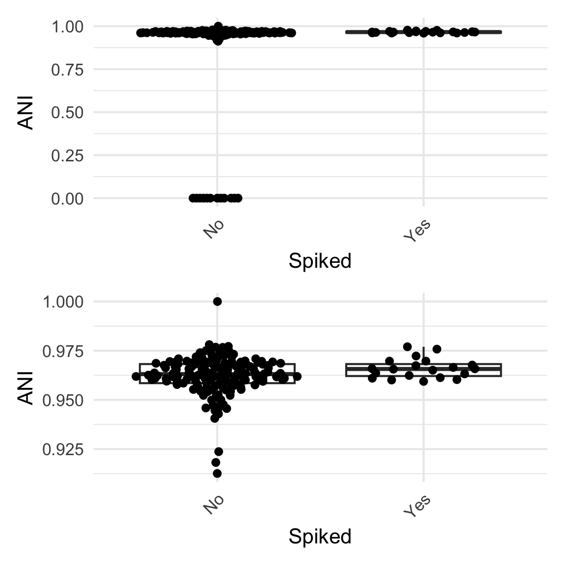
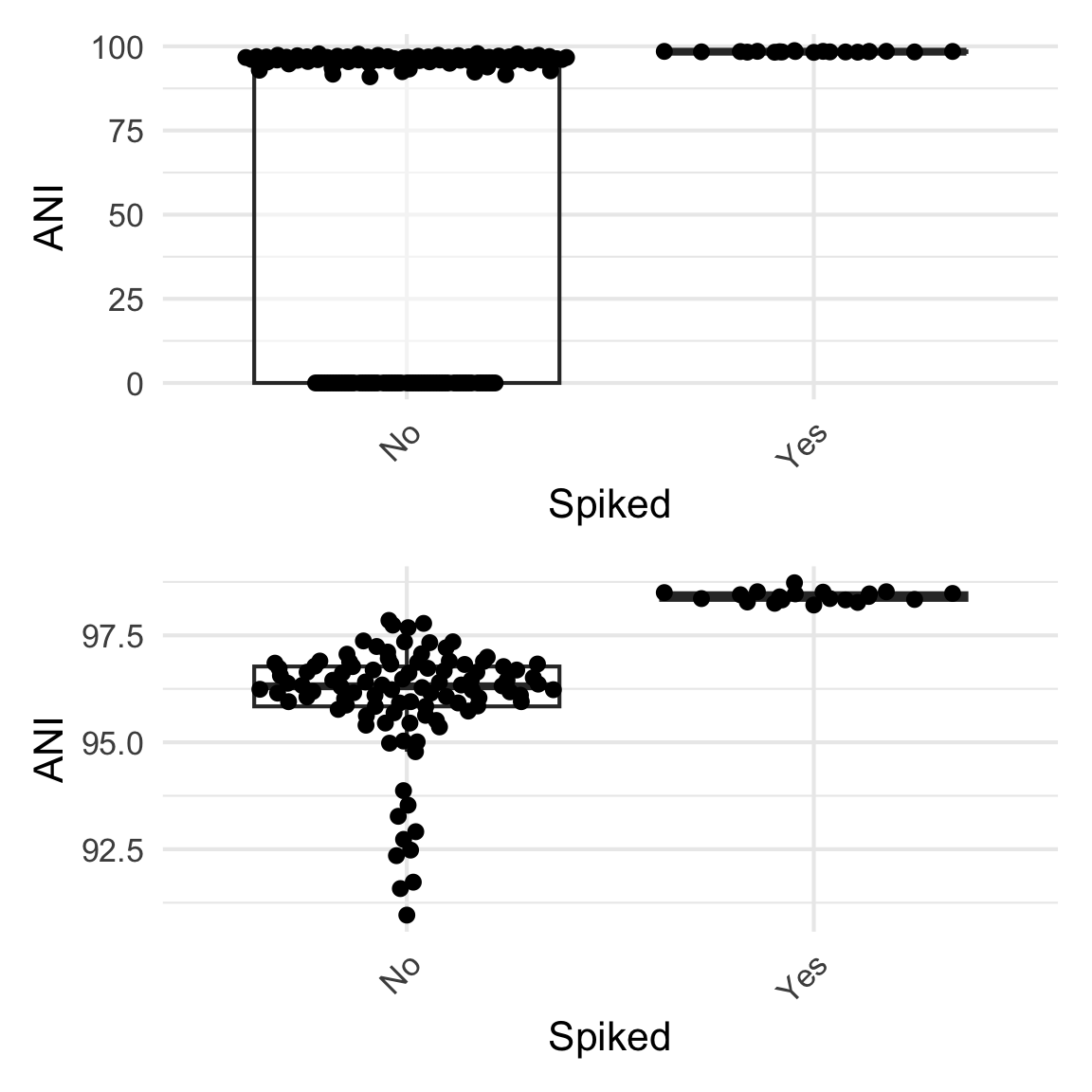
see_boxplot(df_fp)

Show code
see_boxplot(df_tp)

Show code
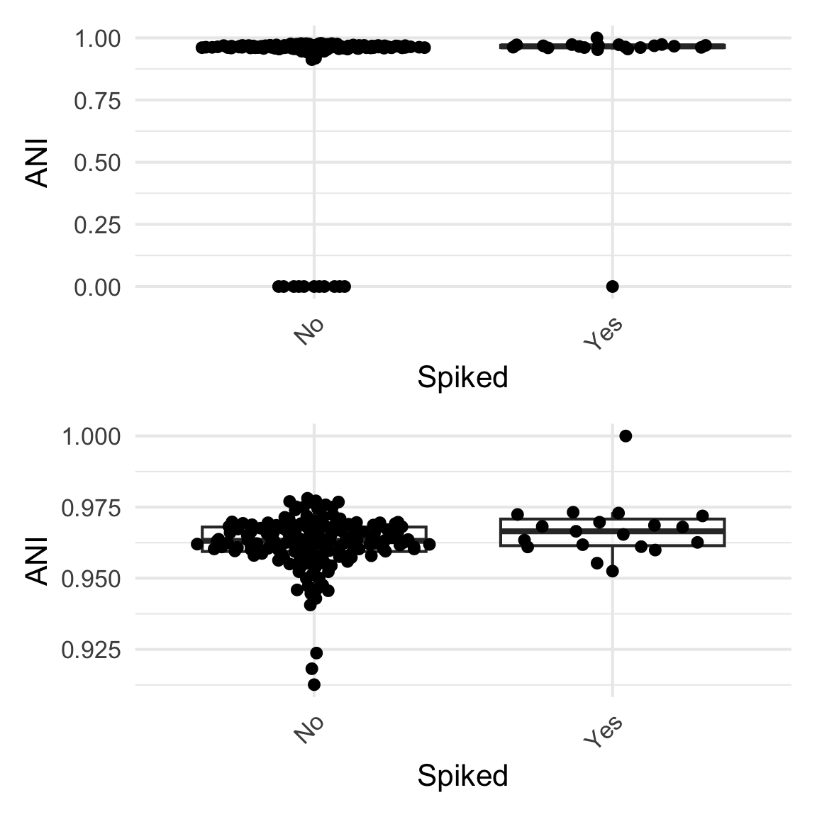
see_boxplot(df_null)

Adjustment Methods

Show code
reset_1 <- function(x, v = 0.99999){
  pmin(x, v)
}

squash <- function(x, eps = 1e-2) {
  x[x > 0] <- x[x > 0] * (1 - 2 * eps) + eps
  x
}

offset <- function(x, eps = 1e-2){
  x[x > 0] <- x[x > 0] - eps
  x
}

rescale_p01p99 <- function(x) {
  out <- x
  is_nonzero <- x != 0
  x_nz <- x[is_nonzero]
  rng <- range(x_nz, na.rm = TRUE)
  rescaled <- (x_nz - rng[1]) / (rng[2] - rng[1])
  out[is_nonzero] <- rescaled * 0.98 + 0.01
  out
}

map_range <- function(x, min_val = 0.9) {
  out <- x
  is_nonzero <- x > 0
  out[is_nonzero] <- (x[is_nonzero] - min_val) / (1 - min_val) * 0.98 + 0.01
  out
}

Compare Adjustments

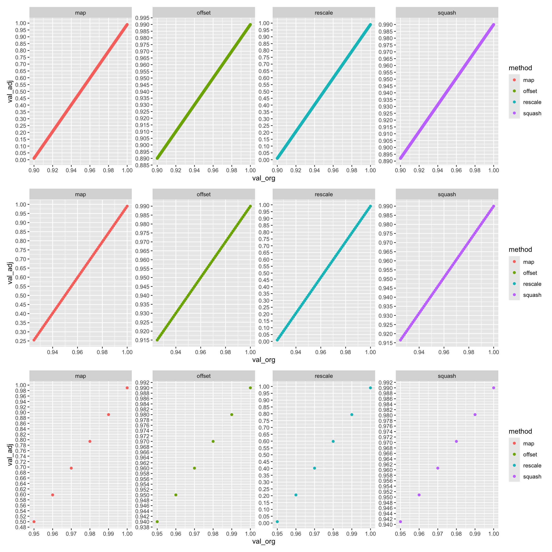
Show code
compare_methods <- function(x){
  plt_df <- data.frame(
    val_org = rep(x, 4),
    method = rep(c("squash", "offset", "rescale", "map"), each = length(x)),
    val_adj = c(squash(x), offset(x), rescale_p01p99(x), map_range(x))
  )

  ggplot(plt_df[plt_df$val_org != 0, ]) + 
    geom_point(aes(x = val_org, y = val_adj, col = method)) + 
    facet_wrap(~method, scales = "free_y", nrow = 1) +
    scale_y_continuous(breaks = scales::pretty_breaks(n = 20)) +
    scale_x_continuous(breaks = scales::pretty_breaks(n = 5))
}
Show code
p1 <- compare_methods(c(0, 9000:10000 / 1e4))
p2 <- compare_methods(c(0, 925:1000 / 1000))
p3 <- compare_methods(c(0, 0.95, 0.96, 0.97, 0.98, 0.99, 1))
wrap_plots(p1 / p2 / p3)

Model Fitting Functions

Show code
fit_and_summary_zib <- function(df, combined_formula = value ~ spiked, design = ~spiked){
  x <- summary(glmmTMB(formula = combined_formula, ziformula = design, data = df, family = beta_family(link = "logit")))
  tmp <- c(x$coefficients$cond[2, c(1,4)], x$coefficients$zi[2, c(1,4)])
  names(tmp) <- c("beta", "p_beta", "z_beta", "z_p_beta")
  tmp
}

fit_and_summary_ob <- function(df, combined_formula = value ~ spiked){
  x <- summary(glmmTMB(formula = combined_formula, data = df, family = ordbeta()))
  tmp <- x$coefficients$cond[2, c(1,4)]
  names(tmp) <- c("beta", "p_beta")
  tmp
}

fit_and_summary_qb <- function(df, combined_formula = value ~ spiked){
  x <- summary(glm(formula = combined_formula, data = df, family = 'quasibinomial'))
  tmp <- x$coefficients[2, c(1,4)]
  names(tmp) <- c("beta", "p_beta")
  tmp
}
Fit All Models

Show code
fit_all <- function(df, dpoint){
  op <- data.frame()

  adj_methods <- list(
    reset_1 = reset_1,
    squash = squash,
    offset = offset,
    rescale = rescale_p01p99,
    map = map_range
  )

  models <- list(
    zib = fit_and_summary_zib,
    ob  = fit_and_summary_ob,
    qb  = fit_and_summary_qb
  )

  for (model_name in names(models)) {
    fit_fun <- models[[model_name]]
    for (adj_name in names(adj_methods)) {
      adj_fun <- adj_methods[[adj_name]]
      df$value <- adj_fun(df$value_)
      tmp <- fit_fun(df)
      op <- rbind(op, data.frame(
        dpoint = dpoint,
        model = model_name,
        adj = adj_name,
        stat = names(tmp),
        vals = unname(tmp)
      ))
    }
  }

  op
}

Run All Comparisons

Show code
op <- rbind(
  fit_all(df_tp, 'tp'),
  fit_all(df_fp, 'fp'),
  fit_all(df_null, 'null')
)

op$log_vals <- with(op, ifelse(stat %in% c("p_beta", "z_p_beta"), -log10(vals), vals))
Warning in ifelse(stat %in% c("p_beta", "z_p_beta"), -log10(vals), vals): NaNs
produced
Show code
op$dpoint <- factor(op$dpoint, levels = c("tp", "fp", "null"))
op$model <- factor(op$model, levels = c("zib", "ob", "qb"))
op$adj <- factor(op$adj, levels = c("reset_1", "squash", "offset", "map", "rescale"))

Visualise Model Effects

Show code
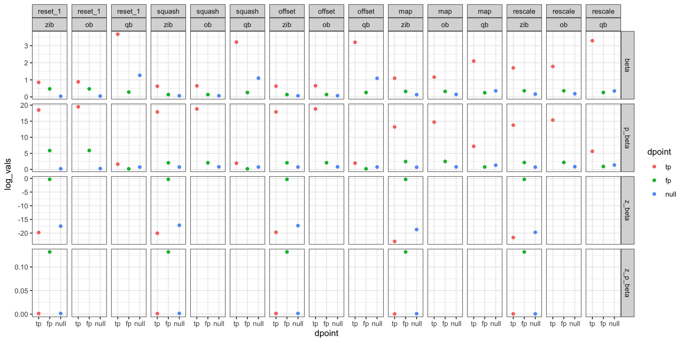
ggplot(op, aes(x = dpoint, y = log_vals, colour = dpoint)) +
  geom_point() +
  facet_grid(stat ~ adj + model, scales = "free_y") +
  scale_fill_brewer(palette = "Set2") +
  theme_bw()