Using gut microbial strains to predict cancer immunotherapy outcomes - a study in rare cancers and melanoma

Load dependencies

Prediction

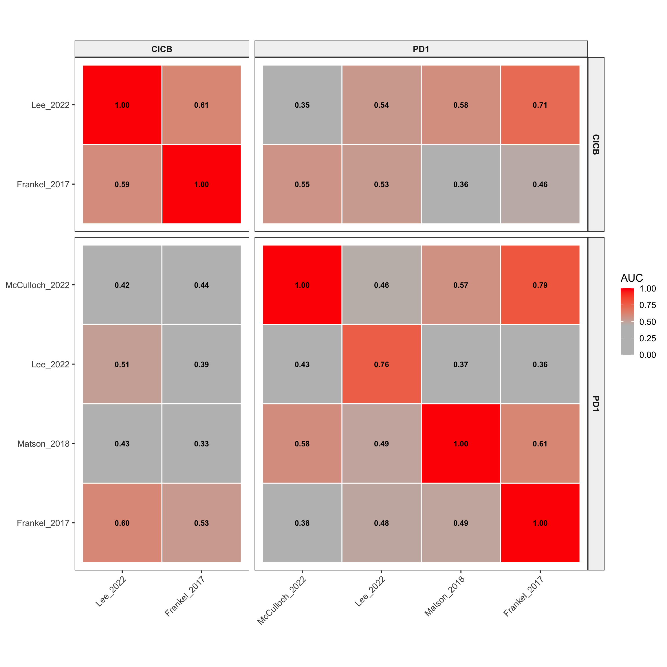
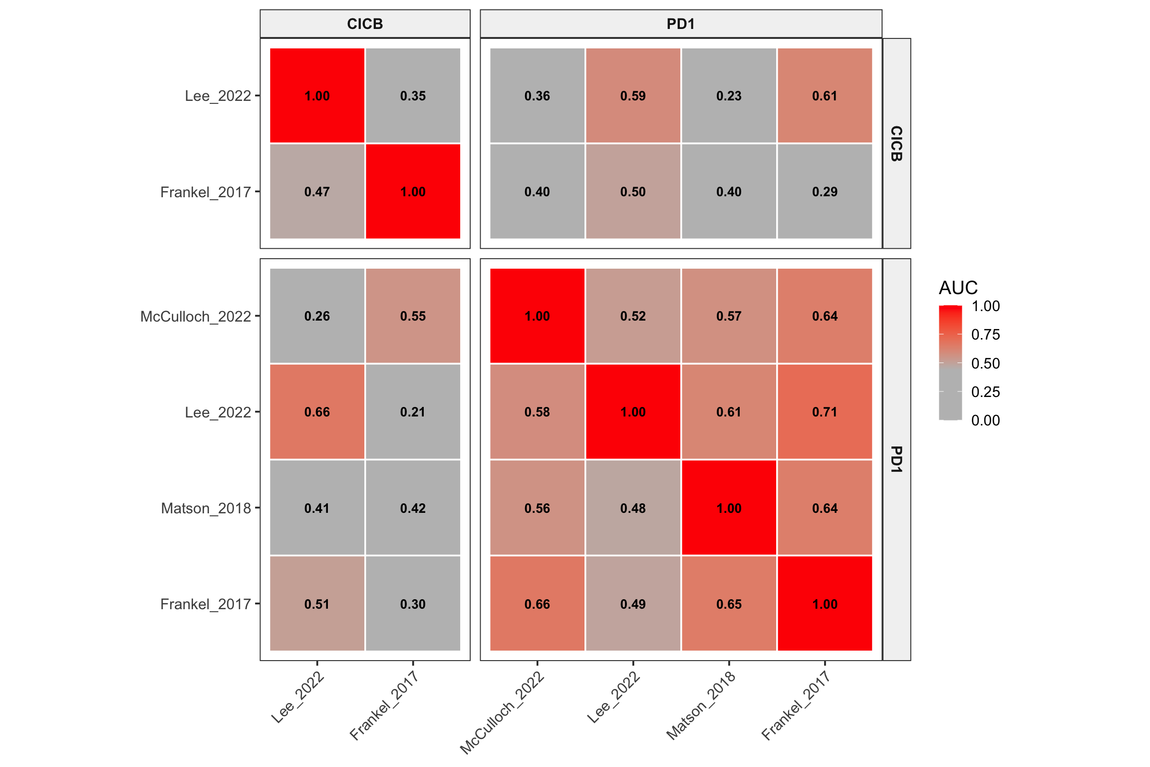
Instead of building a set of predictors using all genomes found through assembly, GTDB, etc. we’ll use StrainSpy with GTDB reference and find a small subset of significant hits in rare cancers and use those strain ANIs to predict outcomes in Melanoma. This avoids dat lekage and attempts to recreate Gunjur et al. Fig 4d using a different approach

Set up some functions

We will be using Elastic net for everything - less resource intensive, but probably less accurate.

run_enet <- function(train_idx, test_idx, meta, sy, feature_names, return_fit = F) {
  
  train_mx <- strainspy::prep_for_prediction(
    sy[, train_idx],
    'RvsP',
    feature_names
  )
  
  cl <- makePSOCKcluster(detectCores() - 1)
  registerDoParallel(cl)
  
  set.seed(1988)
  fit <- caret::train(
    RvsP ~ .,
    data = train_mx,
    method = "glmnet",
    preProcess = c("center", "scale"),
    metric = "ROC",
    trControl = caret::trainControl(
      method = "cv",
      classProbs = TRUE,
      summaryFunction = twoClassSummary,
      savePredictions = "final"
    )
  )
  
  if(return_fit) {
    # If return_fit, we only use the test_idx to see if it has both classes
    return(fit)
  }
  
  
  test_mx <- strainspy::prep_for_prediction(
    sy[, test_idx],
    'RvsP',
    feature_names
  )
  
  # Skip if test labels are all one class
  if (length(unique(test_mx$RvsP)) < 2) {
    warning("Test class only has one type of label")
    return(NA)
  }
  
  
  preds <- predict(fit, test_mx, type = "prob")$R
  roc_obj <- roc(test_mx$RvsP, preds, levels = c("NR","R"))
  as.numeric(auc(roc_obj))
}

print_auc <- function(boot_auc, ret = F){
  point_est <- median(boot_auc)
  ci_lower  <- quantile(boot_auc, 0.025)
  ci_upper  <- quantile(boot_auc, 0.975)
  
  cat("AUC =", round(point_est, 3), "[95% CI:", round(ci_lower, 3), "-", round(ci_upper, 3), "]\n")
  
  if(ret){
    return(c(point_est, ci_lower, ci_upper))
  }
}

evaluate_test_set <- function(fit, test_idx, sy, th_filt_names, B = 1000) {
  if (length(test_idx) == 0) return(c(0, 0, 0))
  
  # Prepare data and predict
  test_mx <- strainspy::prep_for_prediction(sy[, test_idx, drop = FALSE], 'RvsP', th_filt_names)
  pred_probs <- predict(fit, test_mx, type = "prob")$R
  
  nr_idx <- which(test_mx$RvsP == "NR")
  r_idx  <- which(test_mx$RvsP == "R")
  
  n_nr <- length(nr_idx)
  n_r  <- length(r_idx)
  
  # Bootstrap loop
  boot_auc <- replicate(B, {
    # Sample from NR and R separately to maintain exact class proportions
    boot_nr <- sample(nr_idx, size = n_nr, replace = TRUE)
    boot_r  <- sample(r_idx,  size = n_r,  replace = TRUE)
    
    # Combine them into our bootstrap index vector
    boot_idx <- c(boot_nr, boot_r)
    
    # Compute AUC cleanly without worrying about class vanishing
    roc_obj <- roc(test_mx$RvsP[boot_idx], pred_probs[boot_idx], 
                   levels = c("NR", "R"), direction = "<", quiet = TRUE)
    as.numeric(auc(roc_obj))
  })
  
  boot_auc <- boot_auc[!is.na(boot_auc)]
  if (length(boot_auc) == 0) return(c(0, 0, 0))
  
  return(print_auc(boot_auc, ret = TRUE)) # Returns c(bmed, lci, uci)
}


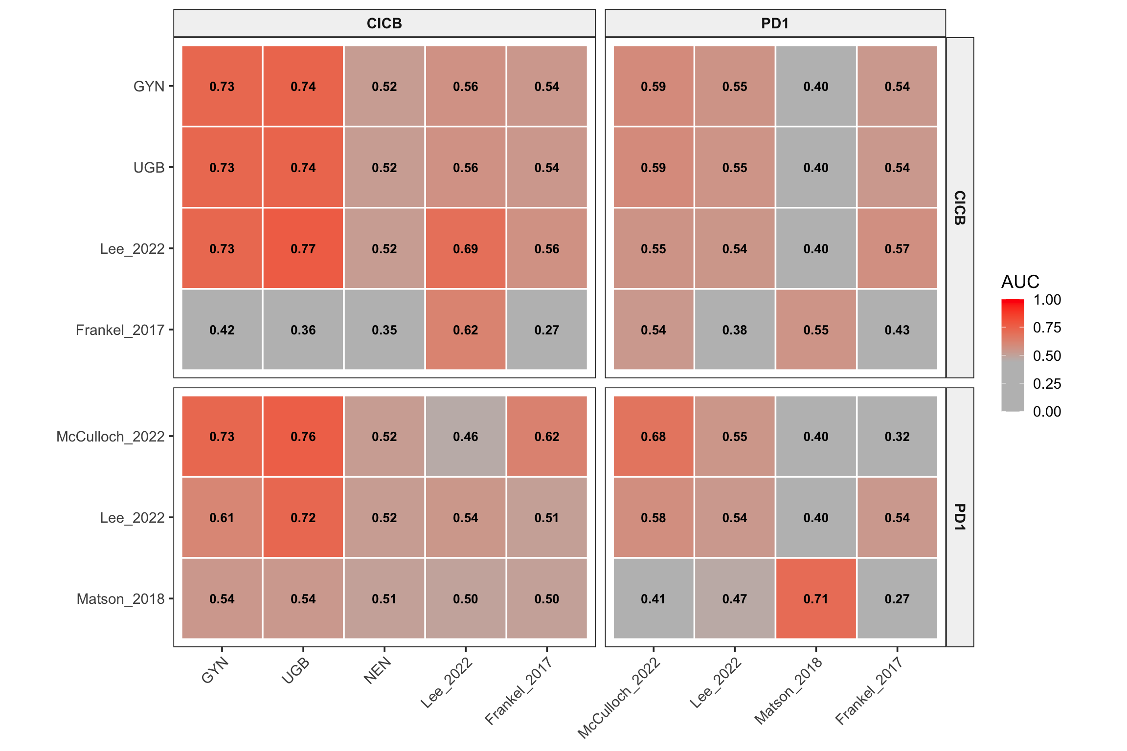
make_paper_heatmap = function(Op){
  ggplot(Op, aes(Test, Train, fill = plot_value)) +
    
    geom_tile(color = "white", linewidth = 0.6) +
    
    geom_text(
      aes(label = ifelse(is.na(plot_value), "", sprintf("%.2f", plot_value))),
      size = 3.5,
      fontface = "bold"
    ) +
    
    scale_fill_gradientn(
      colours = c("grey", "grey", "#ff0000"), 
      values = scales::rescale(c(0.2, 0.55, 1)),
      limits = c(0, 1),
      name = "AUC",
      na.value = "black"
    ) +
    
    coord_fixed() +
    
    facet_grid(
      therapy_train ~ therapy_test,
      scales = "free",
      space = "free"
    ) +
    
    
    theme_bw(base_size = 14) +
    
    theme(
      panel.grid = element_blank(),
      axis.title = element_blank(),
      axis.text.x = element_text(angle = 45, hjust = 1),
      strip.background = element_rect(fill = "grey95"),
      strip.text = element_text(face = "bold")
    )
}

Classic cross prediction

Visualise

study_order = c("GYN", "UGB", "NEN", "McCulloch_2022", "Lee_2022", "Matson_2018", "Frankel_2017")
Op$plot_value <- Op$bmed
Op$plot_value[Op$bmed == 0] <- NA

Op2 <- Op %>%
  filter(Train %in% study_order,
         Test %in% study_order) %>%
  group_by(therapy_train, therapy_test, Train) %>%
  filter(any(!is.na(plot_value))) %>%
  ungroup() %>%
  group_by(therapy_train, therapy_test, Test) %>%
  filter(any(!is.na(plot_value))) %>%
  ungroup()

Op2$Train <- factor(Op2$Train, levels = rev(study_order))  # top → bottom
Op2$Test  <- factor(Op2$Test,  levels = study_order)       # left → right

Op2$plot_value <- Op2$bmed

make_paper_heatmap(Op2)

Load the metadata for rare cancers

# Gunjur et al. data
meta_path_ash <- "./data/ash_pancancer/metadata_full.tsv"
meta_ash <- read.csv(meta_path_ash, sep = '\t') 
meta_ash = cbind(run_acc = meta_ash$run_accession, meta_ash)

# Outcome
meta_ash$RvsP = "R"
meta_ash$RvsP[which(meta_ash$BOR == "PD" | meta_ash$BOR == "cPD")] = "NR" 
meta_ash$RvsP = factor(meta_ash$RvsP, levels = c("NR", "R"))

Load Sylph outputs

sy_ash <- read_sylph("./data/ash_pancancer/combined_q_99.tsv.gz") # q99)

Detected Sylph query output file.

# annoying renames to match meta V sylph file
colnames(sy_ash) <- gsub("_1", "", colnames(sy_ash))
colData(sy_ash)$Sample_file <- gsub("_1", "", basename(colData(sy_ash)$Sample_file))

# Reorder meta_ash 
meta_ash = meta_ash[match(colnames(sy_ash), meta_ash$run_accession), ]
# get rid of SD
rmidx = which(meta_ash$BOR == "SD")
if(length(rmidx) > 0){
  meta_ash = meta_ash[-rmidx, ]
  sy_ash = sy_ash[, -rmidx]
}

sy_ash <- filter_by_presence(sy_ash, min_nonzero = 8) # filter at 10%

Retained 19139 rows after filtering

dim(sy_ash)

[1] 19139    77

# Checks before merging metadata
all(colnames(sy_ash) %in% meta_ash$run_accession)

[1] TRUE

all(meta_ash$run_accession %in% colnames(sy_ash))

[1] TRUE

sy_ash = modify_metadata(sy_ash, meta_ash)

Run StrainSpy

design <- as.formula("~ RvsP + histology_cohort.x + age + sex + BMI") 

save_path <- "output_rds/ASH_zib_q_99_ebp.rds"

if(file.exists(save_path)){
  ZB_fit <- readRDS(save_path)
} else {
  # Run with weak prior for prediction
  ebp = compute_eb_priors(sy_ash, design, nthreads = 10L, low_cutoff = 0, high_cutoff = Inf)
  ZB_fit <- glmZiBFit(sy_ash, design, nthreads = parallel::detectCores(), MAP_prior = ebp)
  saveRDS(ZB_fit, save_path)
}



# These are strainspy predictors from Pancx data
th = top_hits = top_hits(ZB_fit, coef = 2, alpha = 0.05)

Found 167 tophits for RvsPR at alpha = 0.05 using holm 

## !!NB: We can't build a model using melanoma data and predict Ash's data - that will cause data leakage!!
# But we can build a model using Ash's data and predict Melanoma. 

# Since Ash's data is all CICB, we'll do cross testing on individual datasets by running strainspy separately and building models

Load the Melanoma datasets

meta_path <- "./data/ash_pancancer/metadata_full.tsv"
meta_pan <- read.csv(meta_path, sep = '\t') 
meta_pan = cbind(run_acc = meta_pan$run_accession, meta_pan)

# Outcome
meta_pan$RvsP = "R"
meta_pan$RvsP[which(meta_pan$BOR == "PD" | meta_pan$BOR == "cPD")] = "NR" 
meta_pan$RvsP = factor(meta_pan$RvsP, levels = c("NR", "R"))

# Melanoma meta - Thanks, Kshitij+Allyson (20260615)
meta_m = read.csv("data/melanoma_pooled/meta_melanoma_sm.csv")
# meta_m2 = read.csv("data/melanoma_pooled/Clean_metadata_Aug5_Allyson_match_2025.txt", sep = '\t')

##### Let's filter sequences to match with Fig. 4a #####
# see select_melanoma_samples.R
keep_samples = readLines("data/melanoma_pooled/gunjur_samples.txt")
meta_m_filt = meta_m %>% filter(X %in% keep_samples)

meta = rbind(data.frame(X = meta_pan$run_acc, c_type = "RARE", type = meta_pan$histology_cohort.x, therapy_type = "combination", RvsP = meta_pan$RvsP), 
             data.frame(X = meta_m_filt$X, c_type = "MEL", type = meta_m_filt$Study_simplified, therapy_type = meta_m_filt$ICB, RvsP = meta_m_filt$ORR))

meta$therapy_type <- ifelse(meta$therapy_type %in% c("aPD1/aCTLA", "combination"), "CICB", ifelse(meta$therapy_type == "aPD1", "PD1", "other"))
meta$therapy_type[is.na(meta$therapy_type)] = "other" # Get this of the NAs 


sy = read_sylph("./data/melanoma_pooled/combined_q_99.tsv") # q99

Detected Sylph query output file.

# annoying renames to match meta V sylph file
colnames(sy) <- gsub("_1", "", colnames(sy))
colData(sy)$Sample_file <- gsub("_1", "", basename(colData(sy)$Sample_file))

# Reduce sy to only keep the ones we have metadata for
sy = sy[, colnames(sy) %in% meta$X]

# Reorder meta 
meta = meta[match(colnames(sy), meta$X), ]

# Checks before merging metadata
all(colnames(sy) %in% meta$X)

[1] TRUE

all(meta$X %in% colnames(sy))

[1] TRUE

sy = modify_metadata(sy, meta, replace = T)

### Filter and keep Melanoma only
sy_melanoma = sy[,sy$c_type=="MEL"]
# sy_melanoma <- filter_by_presence(sy_melanoma, min_nonzero = 42) # filter at 10%
dim(sy_melanoma)

[1] 45199   224

meta_melanoma = meta[meta$c_type == "MEL", ]

Predict using StrainSpy significant predictors

Build a model using rare cancer data

th_filt <- th[th$Contig_name %in% rownames(sy_melanoma), ] # We are working with just 34 predictors

train_idx <- 1:dim(sy_ash)[2]
fit <- run_enet(train_idx, "", meta_ash, sy_ash, th_filt$Contig_name, return_fit = TRUE)

Prepared data: 77 samples and 167 predictors.

test_dset = unique(sy_melanoma$type)
therapy_types <- c("CICB", "PD1")

B <- 1000
set.seed(1988)

Op <- data.frame()

for (test_dset_nm in test_dset) {
  cat("Training:", "rare", "(", "CICB", ") | Testing set:", test_dset_nm, "\n")
  
  for (test_type in therapy_types) {
    # Determine test indices based on type criteria (preserving your original != 'CICB' logic for 'Other')
    test_idx <- which(sy_melanoma$type == test_dset_nm & sy_melanoma$therapy_type == test_type)
    
    # 4. Evaluate metrics
    if (length(test_idx) > 0) {
      tmp <- evaluate_test_set(fit, sy = sy, test_idx, th_filt$Contig_name, B = B)
      
    } else {
      tmp <- c(NA, NA, NA)
    }
    
    # 5. Append cleanly to output data frame
    Op <- rbind(Op, data.frame(
      Train         = 'rare', 
      Test          = test_dset_nm,
      bmed          = tmp[1], 
      lci           = tmp[2], 
      uci           = tmp[3], 
      therapy_test  = test_type, 
      therapy_train = 'CICB'
    ))
  }
}

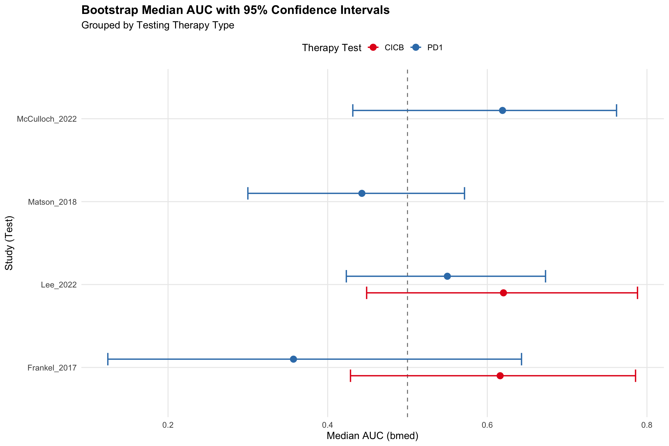
Training: rare ( CICB ) | Testing set: Lee_2022 

Prepared data: 41 samples and 167 predictors.

AUC = 0.62 [95% CI: 0.449 - 0.788 ]

Prepared data: 82 samples and 167 predictors.

AUC = 0.55 [95% CI: 0.423 - 0.673 ]
Training: rare ( CICB ) | Testing set: McCulloch_2022 

Prepared data: 29 samples and 167 predictors.

AUC = 0.619 [95% CI: 0.431 - 0.762 ]
Training: rare ( CICB ) | Testing set: Frankel_2017 

Prepared data: 22 samples and 167 predictors.

AUC = 0.616 [95% CI: 0.429 - 0.786 ]

Prepared data: 11 samples and 167 predictors.

AUC = 0.357 [95% CI: 0.125 - 0.643 ]
Training: rare ( CICB ) | Testing set: Matson_2018 

Prepared data: 24 samples and 167 predictors.

AUC = 0.443 [95% CI: 0.3 - 0.571 ]

ggplot(Op, aes(x = bmed, y = Test, color = therapy_test)) +
  # Adds a dashed reference line at AUC = 0.5 (random chance)
  geom_vline(xintercept = 0.5, linetype = "dashed", color = "gray50") +
  # Draws the CI error bars (dodged so overlapping test points don't clash)
  geom_errorbarh(aes(xmin = lci, xmax = uci), width = 0.3, 
                 position = position_dodge(width = 0.4), size = 0.8) +
  # Draws the median AUC points
  geom_point(position = position_dodge(width = 0.4), size = 3.5) +
  # Formatting & Labels
  scale_color_brewer(palette = "Set1") +
  labs(
    title = "Bootstrap Median AUC with 95% Confidence Intervals",
    subtitle = "Grouped by Testing Therapy Type",
    x = "Median AUC (bmed)",
    y = "Study (Test)",
    color = "Therapy Test"
  ) +
  theme_minimal(base_size = 13) +
  theme(
    panel.grid.minor = element_blank(),
    legend.position = "top",
    plot.title = element_text(face = "bold")
  )

Warning: `geom_errorbarh()` was deprecated in ggplot2 4.0.0.
ℹ Please use the `orientation` argument of `geom_errorbar()` instead.

Warning: Using `size` aesthetic for lines was deprecated in ggplot2 3.4.0.
ℹ Please use `linewidth` instead.
ℹ The deprecated feature was likely used in the ggplot2 package.
  Please report the issue at <https://github.com/tidyverse/ggplot2/issues>.

Warning: Removed 2 rows containing missing values or values outside the scale range
(`geom_point()`).

Training and testing

Visualise

# Try to mimic ash's original figure
# Unfortunately we can't access Simpson and Andrews, everything else is here (and a couple more as well!)
study_order <- c("McCulloch_2022", "Lee_2022", "Matson_2018", "Frankel_2017")

Op$plot_value <- Op$bmed
Op$plot_value[Op$bmed == 0] <- NA

Op2 <- Op %>%
  filter(Train %in% study_order,
         Test %in% study_order) %>%
  group_by(therapy_train, therapy_test, Train) %>%
  filter(any(!is.na(plot_value))) %>%
  ungroup() %>%
  group_by(therapy_train, therapy_test, Test) %>%
  filter(any(!is.na(plot_value))) %>%
  ungroup()

Op2$Train <- factor(Op2$Train, levels = rev(study_order))  # top → bottom
Op2$Test  <- factor(Op2$Test,  levels = study_order)       # left → right

Op2$plot_value <- Op2$bmed

make_paper_heatmap(Op2)

Load data from Gunjur et al using AI

# chatGPT pull from paper
Op4d <- data.frame(
  
  Train = c(
    # CICB → CICB
    rep("CA209-538", 9),
    rep("2022_Simpson", 9),
    rep("2022_Lee", 9),
    rep("2021_Andrews", 9),
    rep("2017_Frankel", 9),
    
    # PD1 → CICB + PD1
    rep("2022_McCulloch", 9),
    rep("2022_Lee_PD1", 9),
    rep("2018_Matson", 9),
    rep("2017_Frankel_PD1", 9)
  ),
  
  Test = c(
    rep(c("CA209-538","2022_Simpson","2022_Lee","2021_Andrews","2017_Frankel",
          "2022_McCulloch","2022_Lee_PD1","2018_Matson","2017_Frankel_PD1"), each = 1)
  ),
  
  bmed = c(
    
    # CICB train → CICB test (5 cols) + CICB→PD1 (4 cols)
    1, 0.67, 0.40, 0.78, 0.75,  0.46, 0.44, 0.58, 0.54,
    0.57, 1, 0.52, 0.59, 0.59,   0.50, 0.52, 0.42, 0.25,
    0.39, 0.64, 1, 0.43, 0.35,   0.36, 0.59, 0.23, 0.61,
    0.72, 0.65, 0.52, 1, 0.63,   0.40, 0.41, 0.46, 0.21,
    0.62, 0.74, 0.47, 0.65, 1,   0.40, 0.50, 0.40, 0.29,
    
    # PD1 train → CICB test (5 cols) + PD1 test (4 cols)
    0.53, 0.29, 0.26, 0.58, 0.55,  1, 0.52, 0.57, 0.64,
    0.42, 0.63, 0.66, 0.22, 0.21,  0.58, 1, 0.61, 0.71,
    0.42, 0.40, 0.41, 0.39, 0.42,  0.56, 0.48, 1, 0.64,
    0.35, 0.33, 0.51, 0.37, 0.30,  0.66, 0.49, 0.65, 1
  )
)

Op4d$therapy_train <- ifelse(grepl("McCulloch|Lee_PD1|Matson|Frankel_PD1", Op4d$Train),
                             "PD1", "CICB")

Op4d$therapy_test <- ifelse(grepl("McCulloch|Lee_PD1|Matson|Frankel_PD1", Op4d$Test),
                            "PD1", "CICB")


Op4d$Train[grep("McCulloch", Op4d$Train)] = "McCulloch_2022"
Op4d$Test[grep("McCulloch", Op4d$Test)] = "McCulloch_2022"

Op4d$Train[grep("Lee", Op4d$Train)] = "Lee_2022"
Op4d$Test[grep("Lee", Op4d$Test)] = "Lee_2022"

Op4d$Train[grep("Matson", Op4d$Train)] = "Matson_2018"
Op4d$Test[grep("Matson", Op4d$Test)] = "Matson_2018"

Op4d$Train[grep("Frankel", Op4d$Train)] = "Frankel_2017"
Op4d$Test[grep("Frankel", Op4d$Test)] = "Frankel_2017"

Op_ash = Op4d %>% filter(Train %in% study_order,
                         Test %in% study_order)

Op_ash$plot_value <- Op_ash$bmed
Op_ash$plot_value[Op_ash$bmed == 0] <- NA

Op_ash2 <- Op_ash %>%
  filter(Train %in% study_order,
         Test %in% study_order) %>%
  group_by(therapy_train, therapy_test, Train) %>%
  filter(any(!is.na(plot_value))) %>%
  ungroup() %>%
  group_by(therapy_train, therapy_test, Test) %>%
  filter(any(!is.na(plot_value))) %>%
  ungroup()

Op_ash2$Train <- factor(Op_ash2$Train, levels = rev(study_order))  # top → bottom
Op_ash2$Test  <- factor(Op_ash2$Test,  levels = study_order)       # left → right

Op_ash2$plot_value <- Op_ash2$bmed

# Original-ish
make_paper_heatmap(Op_ash2)

Build a comparison plot of better visualisation

df_new <- Op2 %>%
  transmute(
    Train,
    Test,
    therapy_train,
    therapy_test,
    cANI = bmed
  )

df_paper <- Op_ash2 %>%
  transmute(
    Train,
    Test,
    therapy_train,
    therapy_test,
    Paper = bmed
  )

df_pair <- inner_join(df_new, df_paper,
                      by = c("Train", "Test", "therapy_train", "therapy_test")) %>%
  filter(Train != Test) %>% # diagonal is annoying and skews everything 
  mutate(therapy_pair = paste(therapy_train, ">", therapy_test))

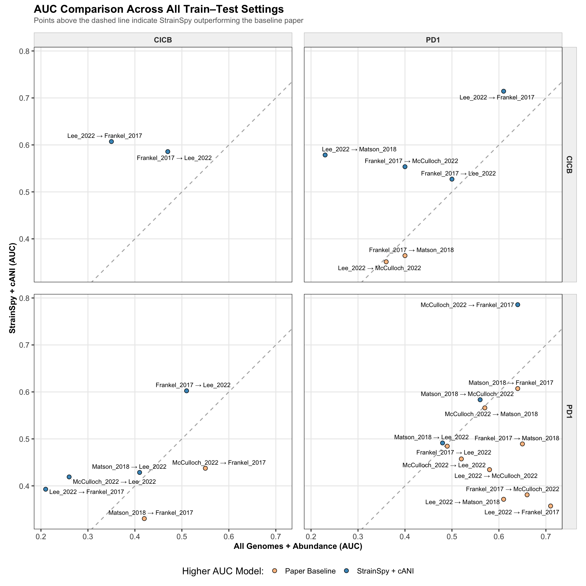
ggplot(df_pair, aes(x = Paper, y = cANI)) +
  # 1. Move the identity line to the background layer so it doesn't cut through points
  geom_abline(slope = 1, intercept = 0, linetype = "dashed", color = "gray60", alpha = 0.8) +
  
  # 2. Consolidated into a single point layer with clean editorial colors
  geom_point(aes(fill = cANI > Paper), shape = 21, color = "black", size = 2.5, stroke = 0.6, alpha = 0.9) +
  
  # 3. Use ggrepel to dynamically push text away from points and other text blocks
  geom_text_repel(
    aes(label = paste0(Train, " → ", Test)),
    size = 3.2,
    box.padding = 0.3,
    point.padding = 0.3,
    segment.color = "gray70",
    segment.size = 0.4,
    min.segment.length = 0, # Always draw lines to points if they move
    max.overlaps = 15       # Increase or set to Inf if you absolutely want every label shown
  ) +
  
  # 4. Custom color scale (Clear visual cue: Blue = StrainSpy won, Orange/Red = Baseline won)
  scale_fill_manual(
    values = c("TRUE" = "#2b8cbe", "FALSE" = "#fdbb84"),
    labels = c("TRUE" = "StrainSpy + cANI", "FALSE" = "Paper Baseline"),
    name = "Higher AUC Model:"
  ) +
  
  # 5. Fix coordinates and facet panels
  coord_equal() +
  facet_grid(therapy_train ~ therapy_test) +
  
  # 6. Use theme_bw for clean panel borders, then finely tune the typography
  theme_bw(base_size = 14) + 
  labs(
    y = "StrainSpy + cANI (AUC)",
    x = "All Genomes + Abundance (AUC)",
    title = "AUC Comparison Across All Train–Test Settings",
    subtitle = "Points above the dashed line indicate StrainSpy outperforming the baseline paper"
  ) +
  theme(
    # Typography
    plot.title = element_text(face = "bold", size = 16, margin = margin(b = 4)),
    plot.subtitle = element_text(size = 11, color = "gray40", margin = margin(b = 12)),
    axis.title = element_text(face = "bold", size = 12),
    
    # Clean up Facet Header Boxes (Strips)
    strip.background = element_rect(fill = "gray95", color = "gray80"),
    strip.text = element_text(face = "bold", size = 11, color = "gray20"),
    
    # Grid adjustments
    panel.grid.minor = element_blank(),
    panel.spacing = unit(1.2, "lines"), # Give facets room to breathe so text doesn't bleed across boxes
    
    # Legend Placement
    legend.position = "bottom",
    legend.box.spacing = unit(0.5, "cm"),
    legend.text = element_text(size = 11)
  )

Prediction using LODO

StrainSpy on the Pan-cancer model (rare + Melanoma)

Load metadata

meta_path <- "./data/ash_pancancer/metadata_full.tsv"
meta_pan <- read.csv(meta_path, sep = '\t') 
meta_pan = cbind(run_acc = meta_pan$run_accession, meta_pan)
# From paper:
# RvsP = CR or PR VS. PD or cPD - excluded patients with a BOR of stable disease (SD) (n=29)

# Outcome
meta_pan$RvsP = "R"
meta_pan$RvsP[which(meta_pan$BOR == "PD" | meta_pan$BOR == "cPD")] = "NR" 
meta_pan$RvsP = factor(meta_pan$RvsP, levels = c("NR", "R"))

# Melanoma meta
meta_m = read.csv("data/melanoma_pooled/Clean_metadata_Aug5_Allyson_match_2025.txt", sep = '\t')


meta = rbind(data.frame(X = meta_pan$run_acc, c_type = "RARE", type = meta_pan$histology_cohort.x, RvsP = meta_pan$RvsP), 
             data.frame(X = meta_m$X, c_type = "MEL", type = meta_m$Study_simplified, RvsP = meta_m$ORR))

Load sylph outputs

sy <- read_sylph("./data/ash_pancancer/merged_pan_melanoma.tsv.gz") # q99)

Detected Sylph query output file.

# annoying renames to match meta V sylph file
colnames(sy) <- gsub("_1", "", colnames(sy))
colData(sy)$Sample_file <- gsub("_1", "", basename(colData(sy)$Sample_file))

# Reorder meta 
meta = meta[match(colnames(sy), meta$X), ]

sy <- filter_by_presence(sy, min_nonzero = 53) # filter at 10%

Retained 19691 rows after filtering

dim(sy)

[1] 19691   526

# Checks before merging metadata
all(colnames(sy) %in% meta$X)

[1] TRUE

all(meta$X %in% colnames(sy))

[1] TRUE

sy = modify_metadata(sy, meta, replace = T)

Fit the univariate model - combined cancers

design <- as.formula("~ RvsP")

save_path <- "output_rds/ASH+mela_zib_q_99_ebp.rds"

if(file.exists(save_path)){
  ZB_fit <- readRDS(save_path)
} else {
  # Run with weak prior for prediction
  ebp = compute_eb_priors(sy, design, nthreads = 10L, low_cutoff = 0, high_cutoff = Inf)
  ZB_fit <- glmZiBFit(sy, design, nthreads = parallel::detectCores(), MAP_prior = ebp)
  saveRDS(ZB_fit, save_path)
}

top_hits(ZB_fit) # No hits - Melanoma is quite heterogenous

Warning in top_hits(ZB_fit): Multiple testing correction using `holm`: No
significant associations detected for coef = 2 at alpha = 0.050000

# A tibble: 0 × 10
# ℹ 10 variables: Contig_name <chr>, Genome_file <chr>, coefficient <dbl>,
#   std_error <dbl>, p_value <dbl>, p_adjust <dbl>, zi_coefficient <dbl>,
#   zi_std_error <dbl>, zi_p_value <dbl>, zi_p_adjust <dbl>

Build a Predictive Species list

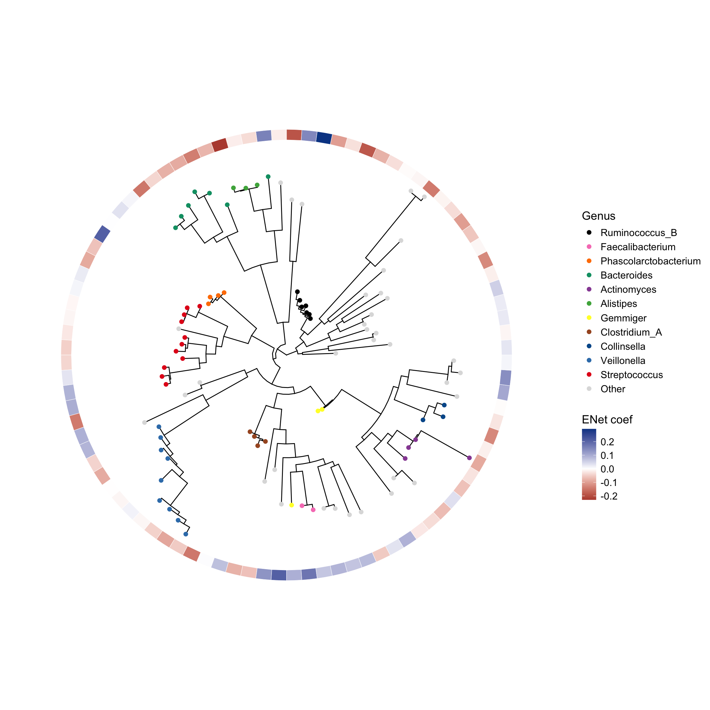
Plot this on a tree

th = top_hits(ZB_fit, alpha = 1)

Found 19691 tophits for RvsPR at alpha = 1 using holm 

th$min_p <- pmin(th$p_value, th$zi_p_value)
th <- th[order(th$min_p), ]
tax_99 = read_taxonomy("data/TAXONOMY/sylph_DB_taxonomy_99.tsv")
th2 = strainspy:::add_tax2tophits(th, tax_99, columns = c("Phylum","Genus","Species"))

# Fit a model using all data and take coefficients
f = 500
fit = run_enet(train_idx = 1:dim(sy)[2], test_idx = "", return_fit = T, meta = meta, sy = sy, feature_names = th$Contig_name[1:f])

Prepared data: 526 samples and 500 predictors.

Warning: from glmnet C++ code (error code -4); Convergence for 4th lambda value
not reached after maxit=100000 iterations; solutions for larger lambdas
returned

coefs <- coef(fit$finalModel, s = fit$bestTune$lambda); coefs = coefs[coefs[,1] != 0,]; coefs = coefs[-1]

# write.table(names(coefs), quote = F, row.names = F, col.names = F, "pancancer_tree_accessions.txt") 

# tree

tree = read.tree("data/ash_pancancer/tree.nwk")
tree$tip.label = unname(sapply(tree$tip.label, function(x) paste(strsplit(x, "_")[[1]][1:2], collapse = "_")))
tree = phytools::midpoint.root(tree)

df <- th2 %>%
  filter(Genome_file %in% names(coefs)) %>%
  transmute(
    tip     = Genome_file,
    Phylum  = Phylum,
    Genus   = Genus,
    Species = Species,
    Coef    = coefs[Genome_file]   # attach coefficients directly
  ) %>%
  arrange(match(tip, tree$tip.label))  # order to match tree

df = as.data.frame(df)

rownames(df) = df$tip

com_gen <- c(
  "Ruminococcus_B",
  "Faecalibacterium",
  "Phascolarctobacterium",
  "Bacteroides",
  "Actinomyces",
  "Alistipes",
  "Gemmiger",
  "Clostridium_A",
  "Collinsella",
  "Veillonella",
  "Streptococcus"
)

genus_cols <- c(
  "#000000", "#f781bf", "#ff7f00",
  "#009E73", "#984ea3", "#4daf4a",
  "#ffff33", "#a65628", "#005999", 
  "#377eb8", "#E41A1C", "#DDDDDD"
)

names(genus_cols) = c(com_gen, "Other")

df$Genus[!df$Genus %in% com_gen] = "Other"

df$Genus = factor(df$Genus, levels = c(com_gen, "Other"))


df = df[rownames(df) %in% tree$tip.label,]
tree = ape::keep.tip(tree,df$tip)

p <- ggtree(tree, layout = "circular")
p$data <- merge(
  p$data,
  df,
  by.x = "label",
  by.y = "tip",
  all.x = TRUE
)

p <- p +
  geom_tippoint(
    aes(color = Genus),
    size = 2
  )  +
  scale_color_manual(
    values = genus_cols,
    name = "Genus"
  )




df_tmp <- data.frame(Coef = df$Coef)
rownames(df_tmp) <- df$tip

p <- gheatmap(
  p,
  df_tmp,
  offset = 0,
  width = 0.05,
  colnames = FALSE
) +
  scale_fill_gradient2(
    high = "#084594",
    mid = "white",
    low = "#99000D",
    midpoint = 0,
    transform = "pseudo_log",
    name = "ENet coef"
  ) +
  theme(
    text = element_text(size = 14),
    legend.title = element_text(size = 14),
    legend.text = element_text(size = 12),
    axis.text = element_text(size = 12)
  )

Scale for y is already present.
Adding another scale for y, which will replace the existing scale.

Scale for fill is already present.
Adding another scale for fill, which will replace the existing scale.

p

Scatter plot with line to see the variation

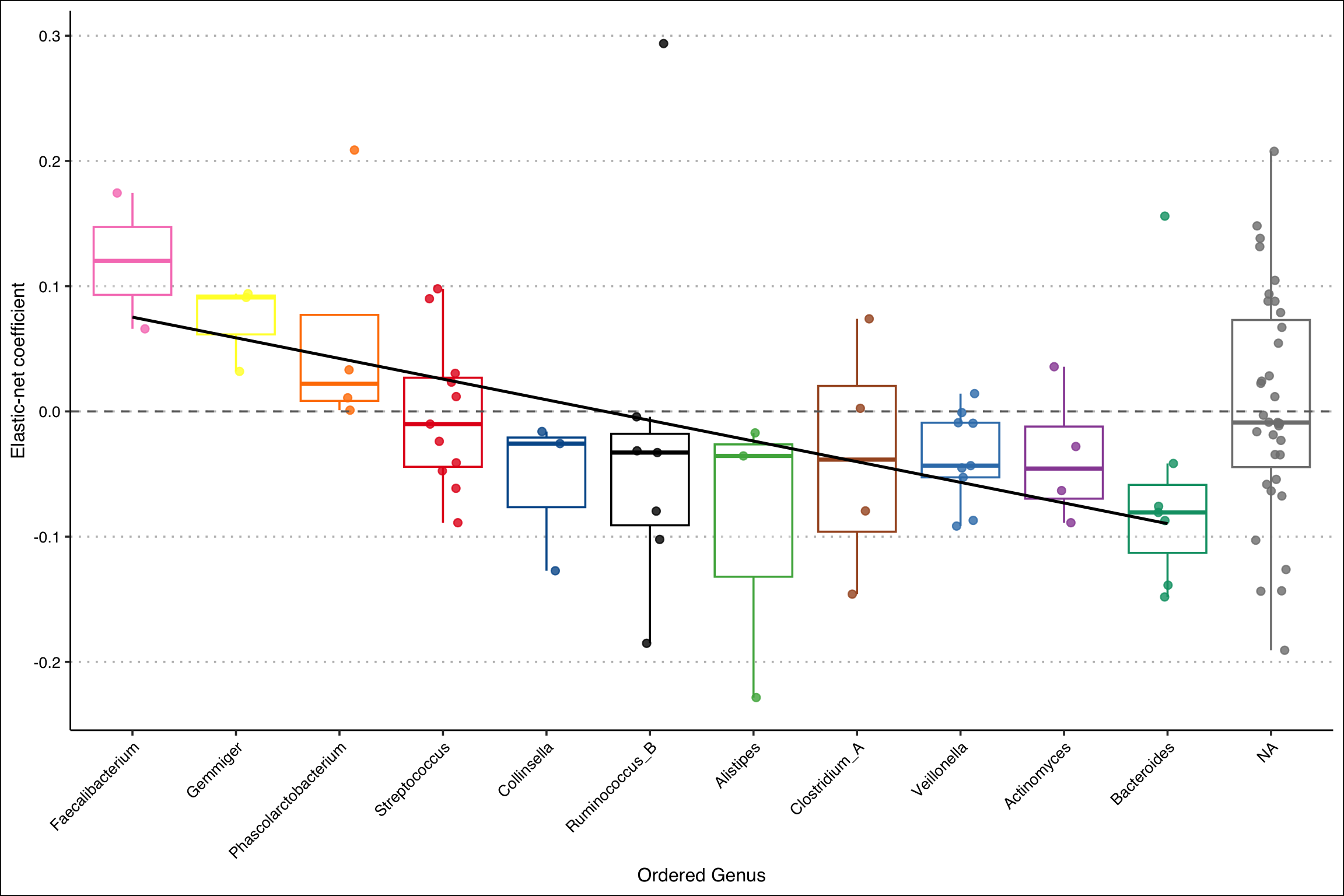
df2 = df
med_df <- df2 %>%
  filter(Genus != "Other") %>%
  group_by(Genus) %>%
  summarise(
    med_coef = median(Coef, na.rm = TRUE),
    .groups = "drop"
  )


scfa_gen <- c(
  # beneficial / SCFA
  "Faecalibacterium",
  "Ruminococcus_B",
  "Phascolarctobacterium",
  "Gemmiger",
  "Eubacterium_F",
  "Bifidobacterium")

genus_order <- df2 %>%
  filter(Genus != "Other") %>%
  group_by(Genus) %>%
  summarise(
    med_coef = median(Coef, na.rm = TRUE),
    .groups = "drop"
  ) %>%
  mutate(
    is_scfa = Genus %in% scfa_gen
  ) %>%
  arrange(
    desc(is_scfa),   # SCFA first
    desc(med_coef)  # then strictly decreasing coef
  ) %>%
  pull(Genus)



med_df$Genus <- factor(med_df$Genus, levels = genus_order)
df2$Genus <- factor(df2$Genus, levels = med_df$Genus[order(med_df$med_coef, decreasing = T)])

fit <- lm(med_coef ~ as.numeric(factor(Genus, levels = med_df$Genus)), data = med_df)

# Coefficients
coef(fit)

                                     (Intercept) 
                                     0.018040411 
as.numeric(factor(Genus, levels = med_df$Genus)) 
                                    -0.004202066 

ggplot(df2, aes(x = Genus, y = Coef, color = Genus, colour = genus_cols)) +
  geom_boxplot(
    outlier.shape = NA,
    alpha = 0.25
  ) +
  geom_jitter(
    width = 0.15,
    size = 2,
    alpha = 0.8
  ) +
  geom_hline(
    yintercept = 0,
    linetype = "dashed",
    colour = "grey40"
  ) +
  geom_smooth(
    data = med_df,
    aes(y = med_coef, group = 1),
    method = "lm",
    se = FALSE,
    colour = "black",
    linewidth = 0.9
  ) +
  scale_color_manual(
    values = genus_cols,
    guide = "none"   # legend already in the tree
  ) +
  labs(
    x = "Ordered Genus",
    y = "Elastic-net coefficient"
  ) +
  ggthemes::theme_clean(base_size = 14) +
  theme(
    axis.text.x = element_text(angle = 45, hjust = 1)
  )

Warning: Duplicated aesthetics after name standardisation: colour

`geom_smooth()` using formula = 'y ~ x'