Analysis of Palleja Antibiotic Exposure data

Load deps

Load metadata and tax

meta = read.table("data/palleja_ab_recovery/metadata.tsv", header = T)
meta$days = factor(meta$days, levels = c(0, 4, 8, 42, 180))
meta$subject = factor(meta$subject)
meta$load = log(meta$g_load) # This is probably better representative given gut microbiome data

conv_design = as.formula('~days + (1 | subject)') # conventional without load adjustment
design = as.formula('~ days + (1|subject) + load')

# tax95 = read_taxonomy(system.file("extdata", "example_taxonomy.tsv.gz", package = "strainspy"))
tax99 = read_taxonomy("data/TAXONOMY/sylph_DB_taxonomy_99.tsv")

Helper functions

cleanup = function(se, meta, min_subj = 3, min_days = 2){
  colnames(se) = gsub("_1", "", colnames(se)) # Reset colnames
  
  
  
  se = modify_metadata(se, meta)
  strainspy:::filter_by_presence_longitudinal(se, subject_col = "subject", 
                                              time_col = "days", 
                                              min_subjects = min_subj, 
                                              min_timepoints = min_days)
}

viz = function(se, fit, tax){
  p1 <- plot_manhattan(fit, taxonomy = tax, aggregate_by_taxa = TRUE)
  p2 <- plot_manhattan(fit, taxonomy = tax, aggregate_by_taxa = FALSE)
  p3 <- plot_volcano(fit, label = TRUE)
  p4 <- plot_ani_dist(
    se,
    phenotype = 'days',
    contigs = top_hits(fit)$Contig_name[1:10],
    show_points = TRUE,
    plot_type = 'box'
  )
  
  # Combine using patchwork
  p1
  p2
  p3
  p4
}

pool_contigs = function(fit, coef = c(2,3,4,5), alpha = 0.05){ # For baseline vs. changes
  return(unique(unlist(sapply(coef, function(cf) top_hits(fit, coef = cf, alpha = alpha)$Contig_name))))
}

Immediate changes following exposure

meta_pre2post = meta[meta$days == 0 | meta$days == 8, ]

se_p = cleanup(read_sylph("data/palleja_ab_recovery/combined_p_95.tsv"), meta)

Detected Sylph profile output file.

Retained 371 rows after subject-aware filtering

se_q = cleanup(read_sylph("data/palleja_ab_recovery/combined_q_99.tsv"), meta)

Detected Sylph query output file.

Retained 15802 rows after subject-aware filtering

Fit to query

save_path <- "output_rds/palleja_zib_q_99.rds"
if(file.exists(save_path)){
  fit_zib_q <- readRDS(save_path)
} else {
  ebp_q = compute_eb_priors(se = se_q, design = as.formula('~ days'),
                            nthreads = parallel::detectCores(), low_cutoff = 0, high_cutoff = Inf, progress = FALSE)
  
  fit_zib_q = glmZiBFit(se_q, conv_design, nthreads = parallel::detectCores(), MAP_prior = ebp_q)
  saveRDS(fit_zib_q, save_path)
}

# Day 0 to day 8
th_q0 = top_hits(fit_zib_q, 3)

Found 484 tophits for days8 at alpha = 0.05 using holm 

th_q0 = comp_ani_diff_and_posthoc_test(se = se_q, fit = fit_zib_q, th = th_q0, progress = FALSE)
th_q = th_q0[is.na(th_q0$Comment), ]

# Reorder so that the highest ani difference ones come on top

th_q <- th_q %>%
  dplyr::arrange(
    desc(abs(ANI_Difference))
  )

th_q = strainspy:::add_tax2tophits(th_q, tax99)
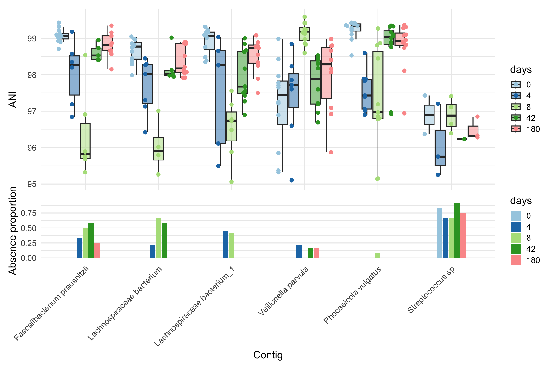
plt_idx = c(1,11,14,35, 62, 169) # Picking different species

plot_ani_dist(se_q, 'days', th_q$Contig_name[plt_idx])

Warning: Removed 96 rows containing non-finite outside the scale range
(`stat_boxplot()`).

# Nice signal here:
# Veillonella sp. - 00100
# Faecalibacterium prausnitzii - 0-1-3-20

Run abundance testing AKA why don’t see see E. coli in ANI testing?

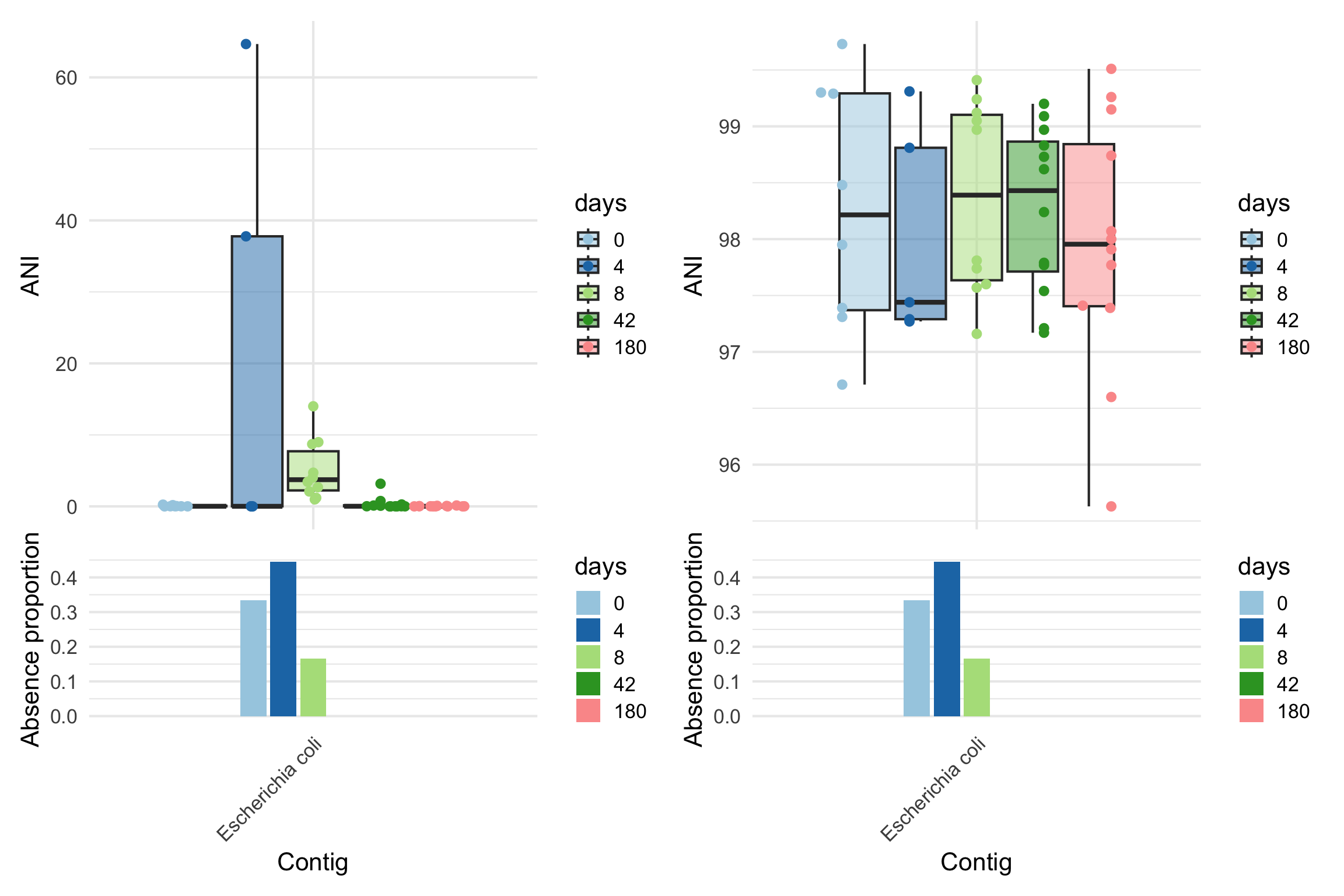
E. coli shows a sharp shift in abundance in the paper (goes up after exposure and then down) - but no change in ANI. Indicative of no strain change or replacement?

se_p95_abund  = cleanup(read_sylph("data/palleja_ab_recovery/combined_p_95.tsv", variable = "Taxonomic_abundance"), meta)

Detected Sylph profile output file.

Retained 371 rows after subject-aware filtering

bug = c("Veillonella", "Klebsiella pneumoniae", "Escherichia coli"); bug_i = 3

p1 = plot_ani_dist(se_p95_abund, 'days',contigs = rownames(se_p95_abund)[grep(bug[bug_i], rownames(se_p95_abund))] , show_points = TRUE,plot_type = 'box')

p2 = plot_ani_dist(se_p, 'days',contigs = rownames(se_p)[grep(bug[bug_i], rownames(se_p))] ,show_points = TRUE,plot_type = 'box')

p1-p2

Warning: Removed 10 rows containing non-finite outside the scale range
(`stat_boxplot()`).
Removed 10 rows containing non-finite outside the scale range
(`stat_boxplot()`).

It seems that relative abundance does have the trend mentioned in the paper, but ANI is unchanged.

Check microbial load vs reported enriched low abundance commensals

summary_df <- meta %>%
  group_by(days) %>%
  summarise(
    mean_log_gload = mean(log(g_load), na.rm = TRUE),
    se_log_gload = sd(log(g_load), na.rm = TRUE) / sqrt(n())
  )

ggplot() +
  geom_line(data = meta, aes(x = as.numeric(days), y = log(g_load), group = subject, color = subject), linewidth = 0.8, alpha = 0.5) +
  geom_point(data = meta, aes(x = as.numeric(days), y = log(g_load), color = subject), size = 3, alpha = 0.8) +
  geom_line(data = summary_df, aes(x = as.numeric(days), y = mean_log_gload), linewidth = 1.2, color = "black") +
  geom_ribbon(data = summary_df, aes(x = as.numeric(days), ymin = mean_log_gload - se_log_gload, ymax = mean_log_gload + se_log_gload), alpha = 0.3, fill = "grey") +
  xlab("Days") +
  ylab("Predicted log microbial load (Galaxy model)") +
  scale_color_manual(values =  c(
    "#D55E00", # reddish-orange  
    "#0072B2", # deep blue  
    "#009E73", # teal/green  
    "#CC79A7", # magenta  
    "#F0E442", # yellow  
    "#E69F00", # orange  
    "#56B4E9", # sky blue  
    "#999999", # gray  
    "#A6761D", # brown  
    "#66CC99", # mint  
    "#CC6666", # muted red  
    "#6699CC"  # muted blue  
  )) +
  scale_x_continuous(breaks = unique(as.numeric(summary_df$days)), labels = unique(summary_df$days)) +
  theme_clean(base_size = 14)

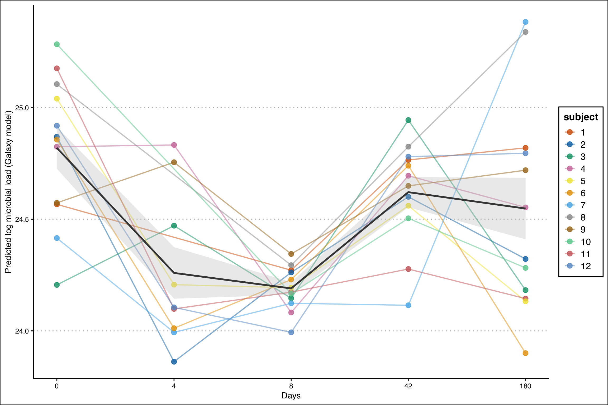
As expected microbial load goes down after antibiotic exposure. Could the relative abundance change in E. coli& be an artifact of this effect?

Perform differential abundance testing

# Helper function
generate_species_plot = function(fit_){
  # Pool the stains that are different at least one day compared to baseline
  plt_dat = plot_ani_dist(se_p95_abund,phenotype = 'days',contigs = pool_contigs(fit_) ,show_points = TRUE,plot_type = 'box', plot = F)
  plt_dat = plt_dat %>% 
    group_by(Contig, days) %>%
    summarise(mean_ANI = mean(ANI, na.rm = TRUE), median_ANI = median(ANI, na.rm = T), .groups = 'drop')
  
  # Thrived
  contigs_thrived <- plt_dat %>%
    group_by(Contig, days) %>%
    tidyr::pivot_wider(names_from = days, values_from = median_ANI) %>%
    filter(`4` > `0` | `8` > `0`) %>%
    pull(Contig) %>%
    unique()
  
  plt_dat$Contig = factor(plt_dat$Contig, levels = unique(plt_dat$Contig)[order(plt_dat$mean_ANI[plt_dat$days == 8], decreasing = T)])
  
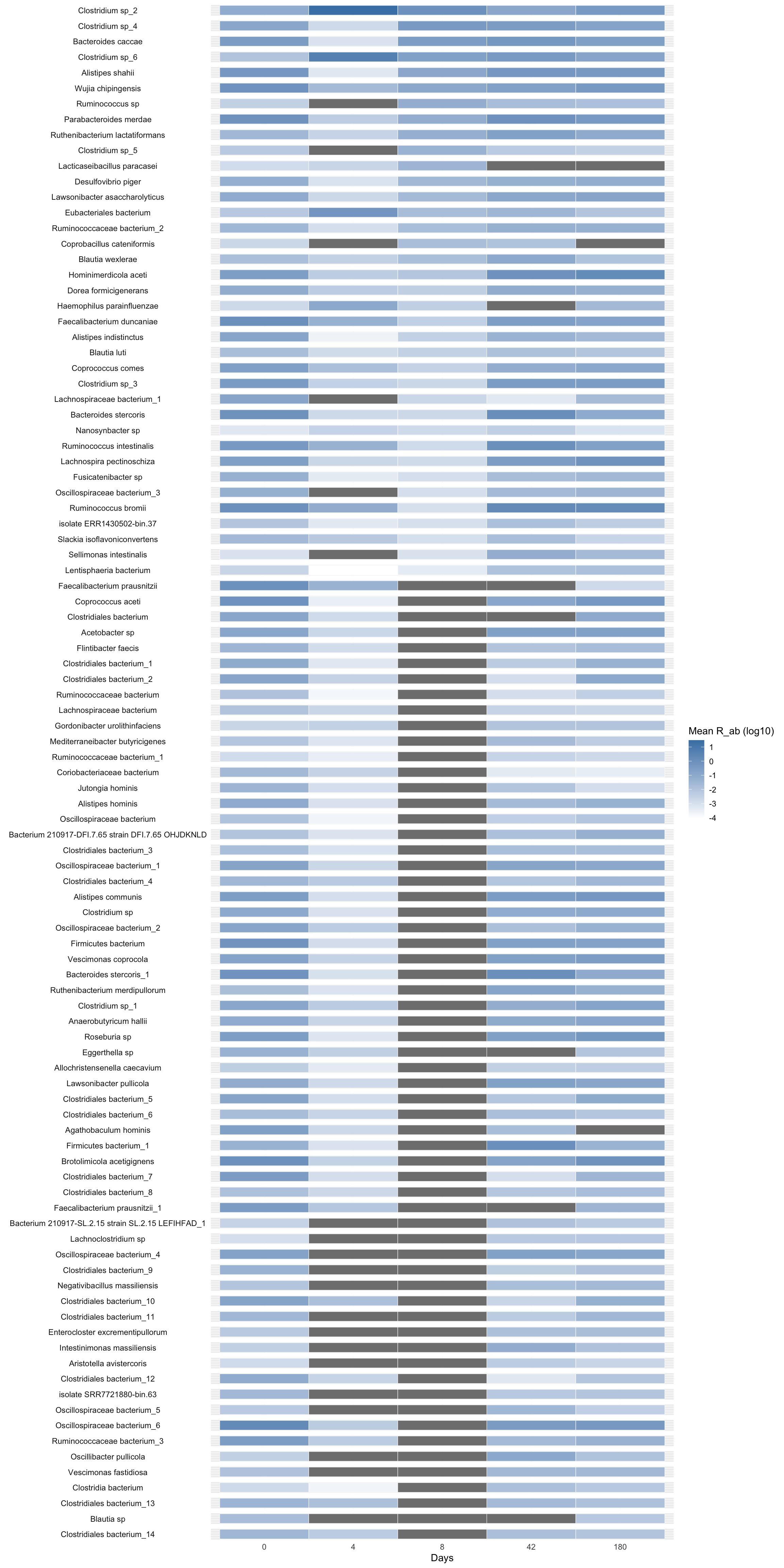
  ggplot(plt_dat, aes(x = factor(days, levels = c(0,4,8,42,180)), y = 1, fill = log10(mean_ANI))) +
    geom_tile(color = "white") +
    facet_wrap(~ Contig, ncol = 1, strip.position = "left") +
    scale_fill_gradient(low = "white", high = "steelblue") +
    labs(x = "Days", y = NULL, fill = "Mean R_ab (log10)") +
    theme_minimal() +
    theme(
      axis.text.y = element_blank(),
      axis.ticks.y = element_blank(),
      strip.text.y.left = element_text(angle = 0)
    )
  
}

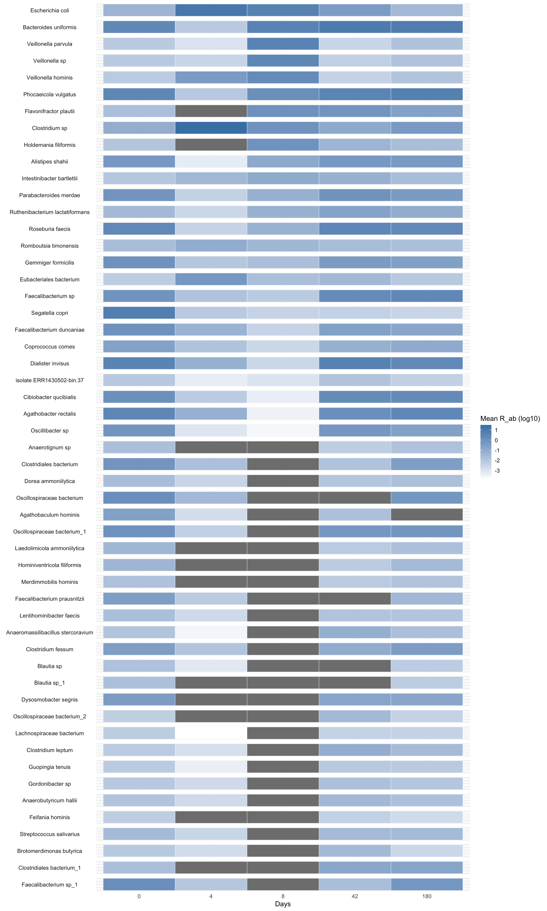
Model without correcting for microbial load

save_path <- "output_rds/palleja_abud_p_95_conv.rds"
if(file.exists(save_path)){
  fit_ab_conv <- readRDS(save_path)
} else {
  fit_ab_conv = abundanceFit(se = se_p95_abund, design = conv_design, nthreads = parallel::detectCores(), transform = 'CLR')
  saveRDS(fit_ab_conv, save_path)
}
generate_species_plot(fit_ab_conv)

Found 29 tophits for days4 at alpha = 0.05 using holm 
Found 42 tophits for days8 at alpha = 0.05 using holm 
Found 18 tophits for days42 at alpha = 0.05 using holm 
Found 8 tophits for days180 at alpha = 0.05 using holm 

Model with load adjustment

save_path <- "output_rds/palleja_abud_p_95_load_adj.rds"
if(file.exists(save_path)){
  fit_ab_load <- readRDS(save_path)
} else {
  fit_ab_load = abundanceFit(se = se_p95_abund, design = design, nthreads = parallel::detectCores(), transform = 'CLR')
  saveRDS(fit_ab_load, save_path)
}

generate_species_plot(fit_ab_load)

Found 18 tophits for days4 at alpha = 0.05 using holm 
Found 20 tophits for days8 at alpha = 0.05 using holm 
Found 13 tophits for days42 at alpha = 0.05 using holm 
Found 3 tophits for days180 at alpha = 0.05 using holm 

No E. coli& detected in either case, and the number of species detected is stable with and without including load as a covariate.

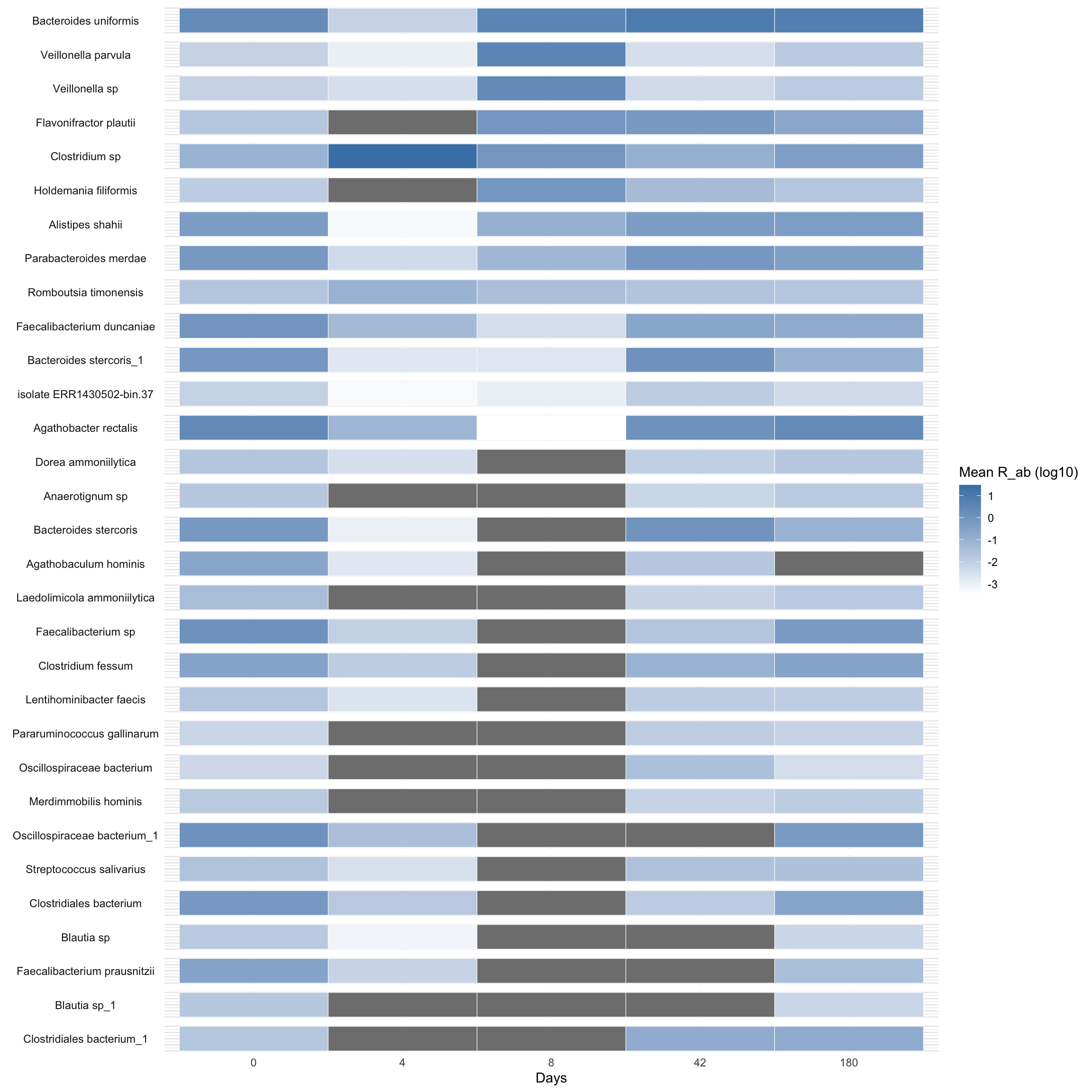
ANI model without load adjustment

save_path <- "output_rds/palleja_fit_p_95_conv.rds"
if(file.exists(save_path)){
  fit_zib_p <- readRDS(save_path)
} else {
  fit_zib_p = glmZiBFit(se = se_p, design = conv_design, nthreads = parallel::detectCores())
  saveRDS(fit_zib_p, save_path)
}

generate_species_plot(fit_zib_p)

Found 59 tophits for days4 at alpha = 0.05 using holm 
Found 16 tophits for days8 at alpha = 0.05 using holm 
Found 24 tophits for days42 at alpha = 0.05 using holm 
Found 19 tophits for days180 at alpha = 0.05 using holm 

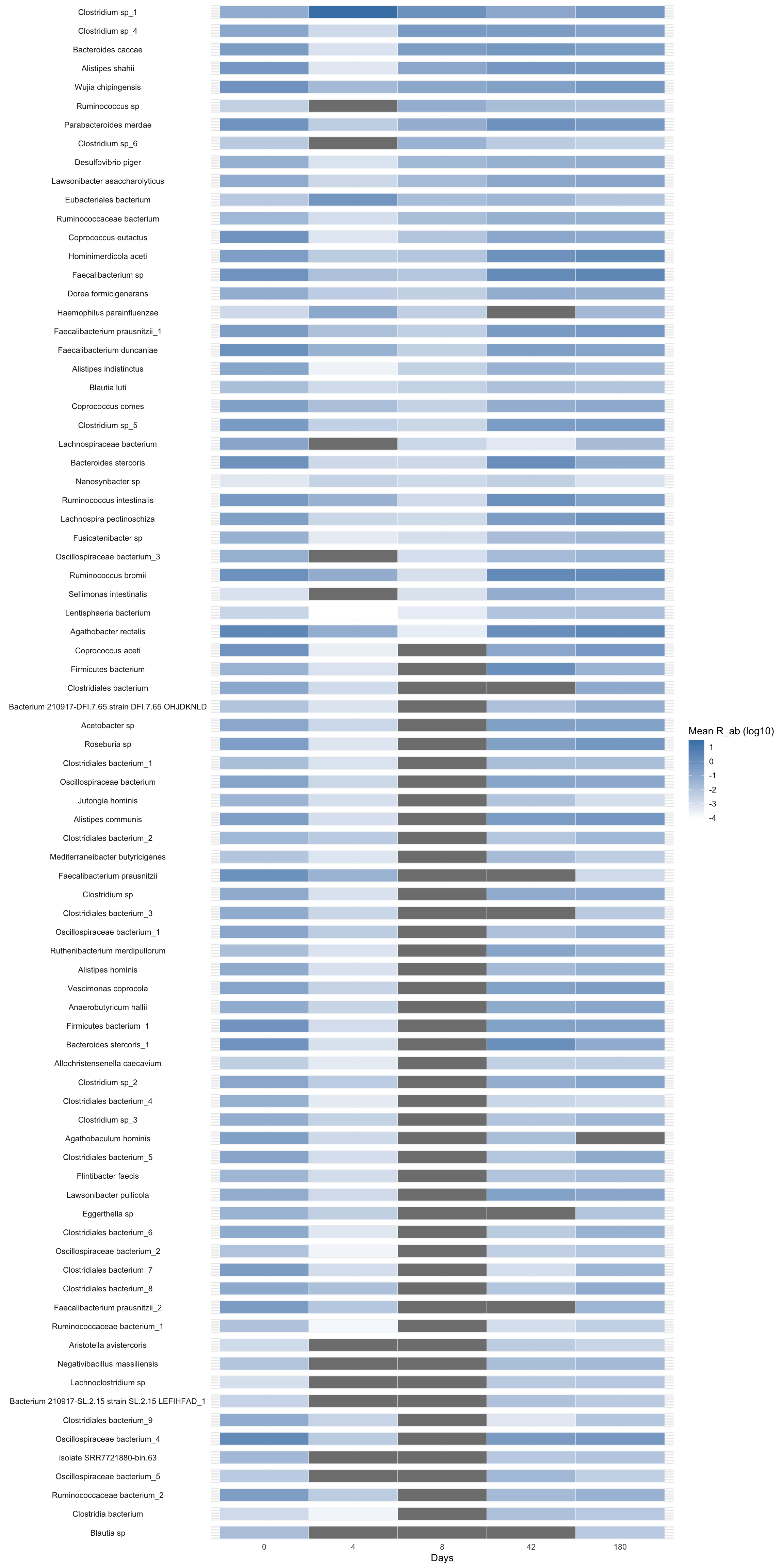
ANI model with load adjustment

save_path <- "output_rds/palleja_fit_p_95_load_adj.rds"
if(file.exists(save_path)){
  fit_zib_p_load <- readRDS(save_path)
} else {
  fit_zib_p_load = glmZiBFit(se = se_p, design = design, nthreads = parallel::detectCores())
  saveRDS(fit_zib_p_load, save_path)
}

generate_species_plot(fit_zib_p_load)

Found 63 tophits for days4 at alpha = 0.05 using holm 
Found 18 tophits for days8 at alpha = 0.05 using holm 
Found 37 tophits for days42 at alpha = 0.05 using holm 
Found 36 tophits for days180 at alpha = 0.05 using holm 

After adjusting for load, we lose many top hits, including E. coli. These were all likely driven by the reduction of overall microbial load.

Paper Figure

Strain emergence or disappearance

Let’s redo top hist using very permissive settings, i.e., use BH and alpha = 0.05. After all, these are still significant after correcting for multiple testing.

th2 = top_hits(fit_zib_q, coef = 2, method = "BH")

Found 4222 tophits for days4 at alpha = 0.05 using BH 

th2_ph = comp_ani_diff_and_posthoc_test(se_q, fit_zib_q, th2, nthreads = parallel::detectCores(), progress = FALSE)
th2 = th2_ph[is.na(th2_ph$Comment) | th2_ph$hit_component == "both",,]; rownames(th2) = NULL
th2 = strainspy:::add_tax2tophits(th2, tax99, columns = c("Phylum", "Genus", "Species"))

th3 = top_hits(fit_zib_q, coef = 3, method = "BH")

Found 7988 tophits for days8 at alpha = 0.05 using BH 

th3_ph = comp_ani_diff_and_posthoc_test(se_q, fit_zib_q, th3, nthreads = parallel::detectCores(), progress = FALSE)
th3 = th3_ph[is.na(th3_ph$Comment) | th3_ph$hit_component == "both",,]
th3 = strainspy:::add_tax2tophits(th3, tax99, columns = c("Phylum", "Genus", "Species"))

th4 = top_hits(fit_zib_q, coef = 4, method = "BH")

Found 646 tophits for days42 at alpha = 0.05 using BH 

th4_ph = comp_ani_diff_and_posthoc_test(se_q, fit_zib_q, th4, nthreads = parallel::detectCores(), progress = FALSE)
th4 = th4_ph[is.na(th4_ph$Comment) | th4_ph$hit_component == "both",]
th4 = strainspy:::add_tax2tophits(th4, tax99, columns = c("Phylum", "Genus", "Species"))

th5 = top_hits(fit_zib_q, coef = 5, method = "BH")

Found 480 tophits for days180 at alpha = 0.05 using BH 

th5_ph = comp_ani_diff_and_posthoc_test(se_q, fit_zib_q, th5, nthreads = parallel::detectCores(), progress = FALSE)
th5 = th5_ph[is.na(th5_ph$Comment) | th5_ph$hit_component == "both",,]
th5 = strainspy:::add_tax2tophits(th5, tax99, columns = c("Phylum", "Genus", "Species"))

top_hits = rbind( data.frame(strainspy:::add_tax2tophits(th2, tax99, columns = c("Phylum", "Genus", "Species")), day = 4),   # day 4
                  data.frame(strainspy:::add_tax2tophits(th3, tax99, columns = c("Phylum", "Genus", "Species")), day = 8),   # day 8
                  data.frame(strainspy:::add_tax2tophits(th4, tax99, columns = c("Phylum", "Genus", "Species")), day = 42),  # day 42
                  data.frame(strainspy:::add_tax2tophits(th5, tax99, columns = c("Phylum", "Genus", "Species")), day = 180)) # day 180


#### Some stats for the paper results ###

# Depletion counts right after exposure
th_depletion = rbind(th2[th2$hit_component == "zi" | th2$hit_component ==  "both",],
                     th3[th3$hit_component == "zi" | th3$hit_component ==  "both",] )
length(unique(th_depletion$Species))

[1] 1140

length(unique(th_depletion$Genus))

[1] 96

th_turnover = rbind(th2[th2$hit_component == "beta" | th2$hit_component ==  "both",],
                     th3[th3$hit_component == "beta" | th3$hit_component ==  "both",] )
length(unique(th_turnover$Species))

[1] 282

length(unique(th_turnover$Genus))

[1] 60

# Recovery
th_recovery = rbind(th4[th4$hit_component == "zi" | th4$hit_component ==  "both",],
                     th5[th5$hit_component == "zi" | th5$hit_component ==  "both",] )
length(unique(th_recovery$Species))

[1] 1

length(unique(th_recovery$Genus))

[1] 1

th_rec_turnover = rbind(th4[th4$hit_component == "beta" | th4$hit_component ==  "both",],
                     th5[th5$hit_component == "beta" | th5$hit_component ==  "both",] )
length(unique(th_rec_turnover$Species))

[1] 96

length(unique(th_rec_turnover$Genus))

[1] 46

contigs_to_pull = unique(top_hits$Contig_name)
asy = SummarizedExperiment::assay(se_q)
asy = as.matrix(asy[unname(sapply(contigs_to_pull, function(x) which(x == rownames(asy)))),])

ani_long <- as.data.frame(asy) %>%
  tibble::rownames_to_column("Contig_name") %>%
  pivot_longer(-Contig_name, names_to = "run_accession", values_to = "ANI") %>%
  left_join(meta %>% select(run_accession, subject, days), by = "run_accession") %>%
  mutate(
    Species = top_hits$Species[match(Contig_name, top_hits$Contig_name)],
    Genus   = top_hits$Genus[match(Contig_name, top_hits$Contig_name)]
  )

ani_filtered <- ani_long %>%
  group_by(subject, Contig_name) %>%
  # Keep only those with at least one non-zero ANI for that subject
  filter(any(ANI != 0)) %>%
  ungroup()


# look at zeros
non_zero_counts <- ani_filtered %>%
  group_by(subject, Genus, days) %>%
  summarise(
    n_zeros   = sum(ANI != 0),
    n_total   = n(),
    prop_zero = n_zeros / n_total,
    n_contigs = n_distinct(Contig_name),
    .groups = "drop"
  ) %>%
  group_by(Genus, days) %>%
  summarise(
    mean_prop_zeros = mean(prop_zero),
    se_prop_zeros   = sd(prop_zero) / sqrt(n()),
    mean_zeros      = mean(n_zeros),
    se_zeros        = sd(n_zeros) / sqrt(n()),
    n_contigs_total = sum(n_contigs),
    n_subjects      = n_distinct(subject),
    .groups = "drop"
  )

Use a weighted sum to detect most affected strains

# Define your kernel for depletion
# Days: 0, 4, 8, 42, 180
# Weights: 1, -1, -1, 1, 1 (High score = Depletion at days 4 & 8)
depletion_kernel <- c(1, -1, -1, 1, 1)
ani_filtered_ <- ani_filtered
ani_filtered_$days = as.numeric(ani_filtered_$days)
# Ensure data is complete and compute scores per subject
strain_stats <- ani_filtered_ %>%
  complete(nesting(Contig_name, Genus, Species, subject), 
           days = c(0, 4, 8, 42, 180), 
           fill = list(ANI = 0)) %>%
  arrange(days) %>%
  group_by(subject, Contig_name, Genus, Species) %>%
  summarise(
    depletion_score = sum(ANI * depletion_kernel),
    .groups = "drop"
  ) %>%
  # Now aggregate across subjects
  group_by(Contig_name, Genus, Species) %>%
  summarise(
    avg_score = mean(depletion_score, na.rm = TRUE),
    sd_score = sd(depletion_score, na.rm = TRUE),
    n_subjects = n(), # Useful to see if the strain was present in all subjects
    .groups = "drop"
  ) %>%
  arrange(desc(avg_score))

Warning: There were 96034 warnings in `summarise()`.
The first warning was:
ℹ In argument: `depletion_score = sum(ANI * depletion_kernel)`.
ℹ In group 1: `subject = 1`, `Contig_name = "AFYM01000001.1 Lacticaseibacillus
  casei A2-362 ctg001_00010, whole genome shotgun sequence"`, `Genus =
  "Lacticaseibacillus"`, `Species = "Lacticaseibacillus paracasei"`.
Caused by warning in `ANI * depletion_kernel`:
! longer object length is not a multiple of shorter object length
ℹ Run `dplyr::last_dplyr_warnings()` to see the 96033 remaining warnings.

Visualise interesting variations of species within genera

genus_dist = function(selected_genera){ 
  selected_species = unique(ani_filtered$Species[ani_filtered$Genus == selected_genera])
  # get genera counts in the database
  species_totals <- tax99 %>%
    filter(Species %in% selected_species) %>%
    distinct(Species, Genome) %>%    # unique strain × genus pairs
    group_by(Species) %>%
    summarize(total_strains = n(), .groups = "drop") %>%
    complete(Species = selected_species, fill = list(total_strains = 0))
  
  day_levels <- c("0","4","8","42","180") 
  
  presence_df <- ani_filtered %>%
    filter(Species %in% selected_species) %>%
    mutate(days = factor(as.character(days), levels = day_levels),
           present = ANI > 95) %>%
    # count unique contig names per Genus x subject x day where present == TRUE
    group_by(Species, subject, days) %>%
    summarize(n_strains = n_distinct(Contig_name[present]), .groups = "drop")
  
  
  prop_df <- presence_df %>%
    left_join(species_totals, by = "Species") %>%
    mutate(
      # avoid division by zero: if genus has zero total strains, produce NA
      prop_of_species = if_else(total_strains > 0,
                                n_strains / total_strains,
                                NA_real_)
    )
  
  baseline <- prop_df %>%
    group_by(Species, subject) %>%
    summarize(
      prop0 = max(prop_of_species, na.rm = TRUE),   # highest proportion across all days
      .groups = "drop"
    )
  
  prop_df2 <- prop_df %>%
    left_join(baseline, by = c("Species", "subject"))
  
  prop_df2 <- prop_df2 %>%
    mutate(
      ratio = if_else(!is.na(prop0) & prop0 > 0,
                      prop_of_species / prop0,
                      NA_real_),      # baseline-0 subjects → NA
      ratio = pmin(ratio, 1)   # cap at 1 so colour means "as present as baseline"
    )
  summary_ratio <- prop_df2 %>%
    group_by(Species, days) %>%
    summarize(
      mean_ratio = mean(ratio, na.rm = TRUE),
      se_ratio   = sd(ratio, na.rm = TRUE) / sqrt(sum(!is.na(ratio))),
      n_subj     = sum(n_strains>0),
      .groups = "drop"
    ) %>%
    mutate(days = factor(as.character(days), levels = c("0","4","8","42","180")))
  
  # Order genera by effect (optional)
  order_species <- summary_ratio %>% filter(days == "8") %>% arrange(mean_ratio) %>% pull(Species) %>% unique()
  summary_ratio <- summary_ratio %>% mutate(Species = factor(Species, levels = rev(order_species)))
  
  # Plot: white -> single colour; limits [0,1]; NA and 0 appear white
  ggplot(summary_ratio, aes(x = days, y = Species, fill = n_subj)) +
    geom_tile(color = "grey90", size = 0.3) +
    geom_text(aes(label = sprintf("%d", n_subj)),
              size = 6) +
    scale_fill_gradient(
      low = "white",
      high = "#2A6EBBFF",    # pick a single strong colour
      limits = c(0, 12),
      na.value = "white",
      name = "Strains Present"
    ) +
    labs(x = "Days", y = NULL) +
    theme_minimal(base_size = 15) +
    theme(panel.grid = element_blank(),
          axis.text.x = element_text(angle = 45, hjust = 1))
}

# Few strong signals to see here:

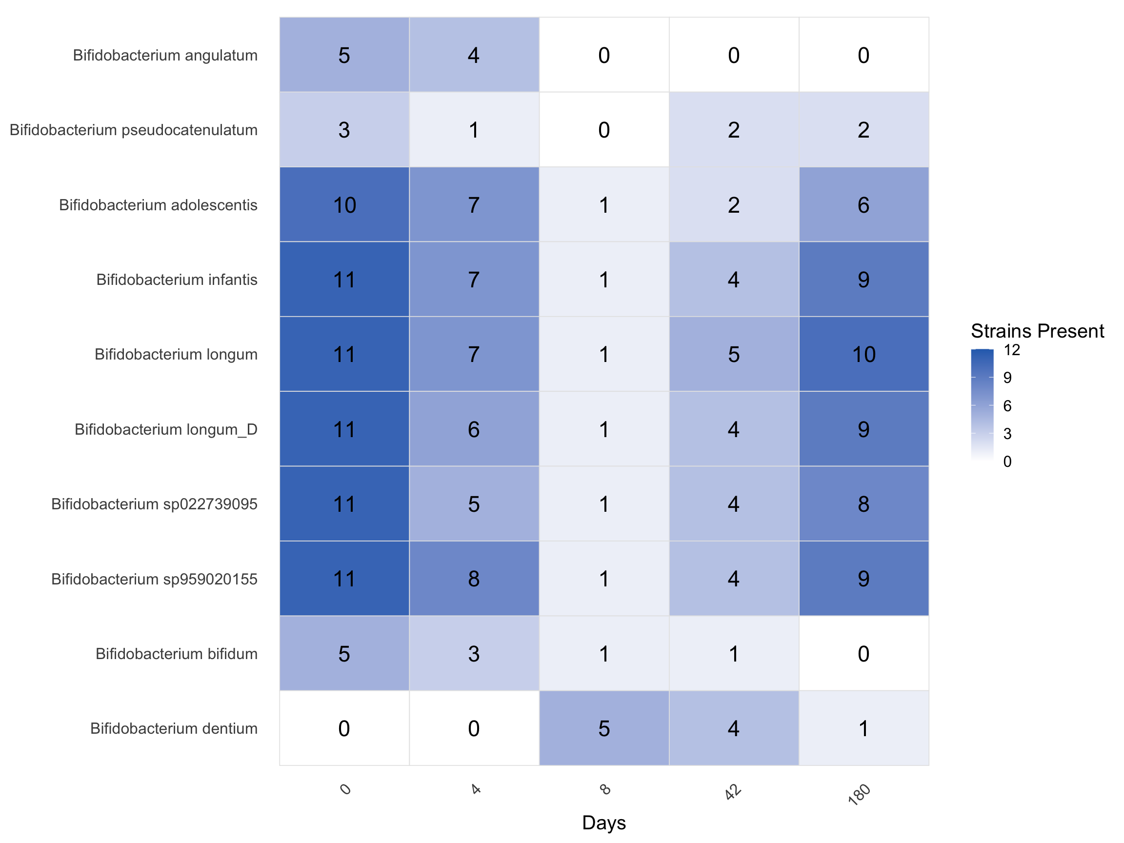
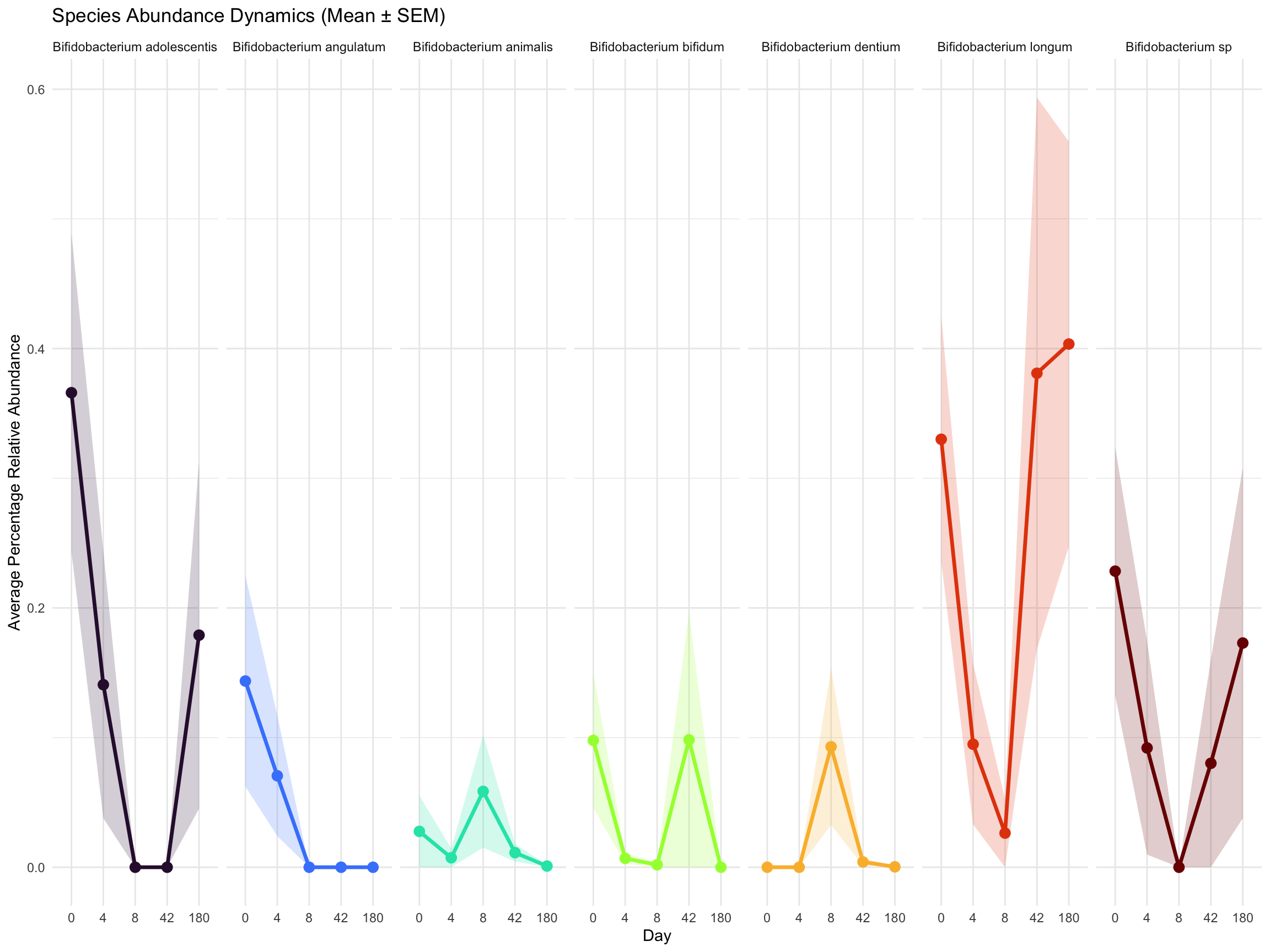
# B. dentium goes up while others go down and slowly recover
genus_dist("Bifidobacterium")

Warning: Using `size` aesthetic for lines was deprecated in ggplot2 3.4.0.
ℹ Please use `linewidth` instead.

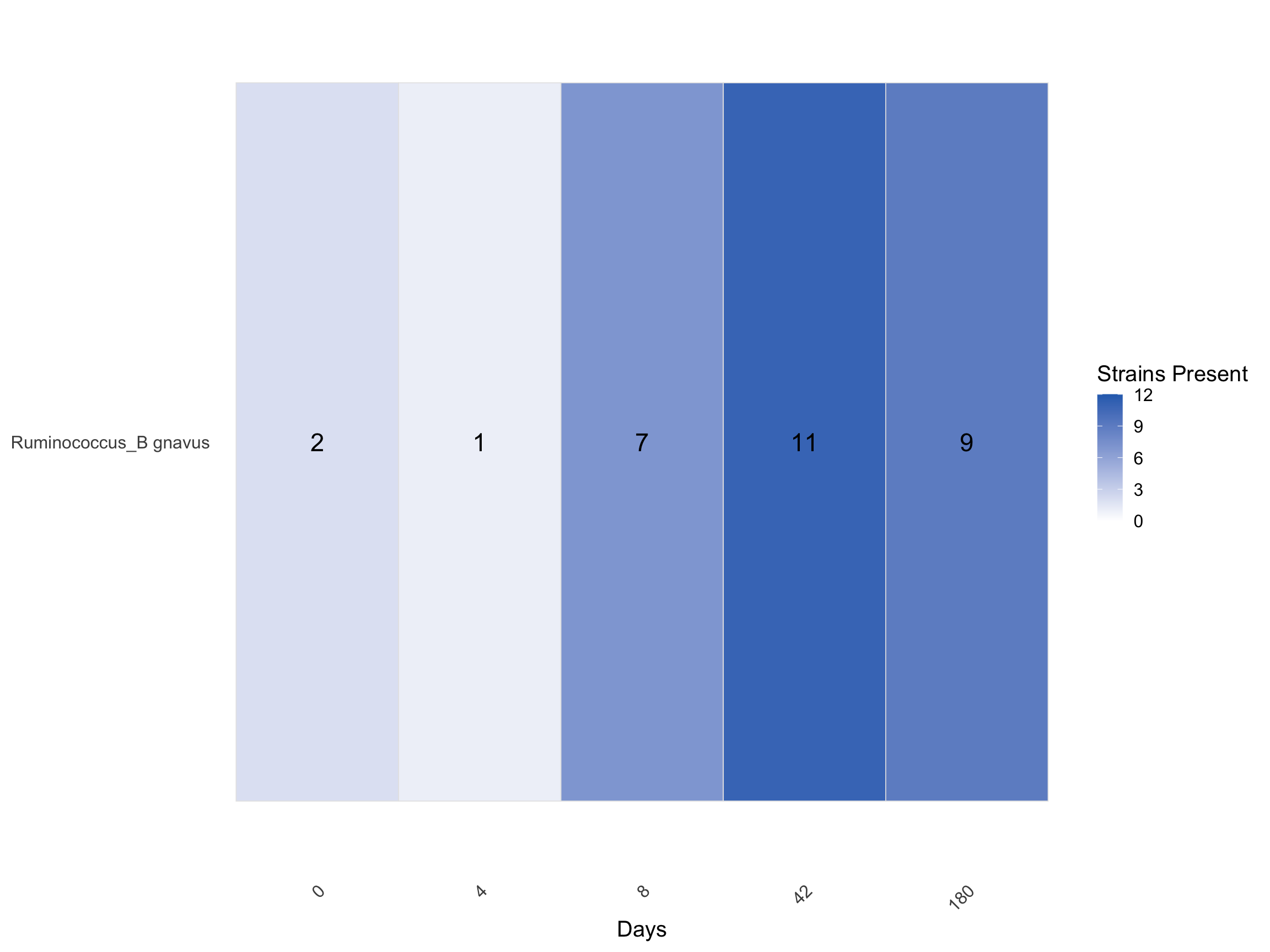
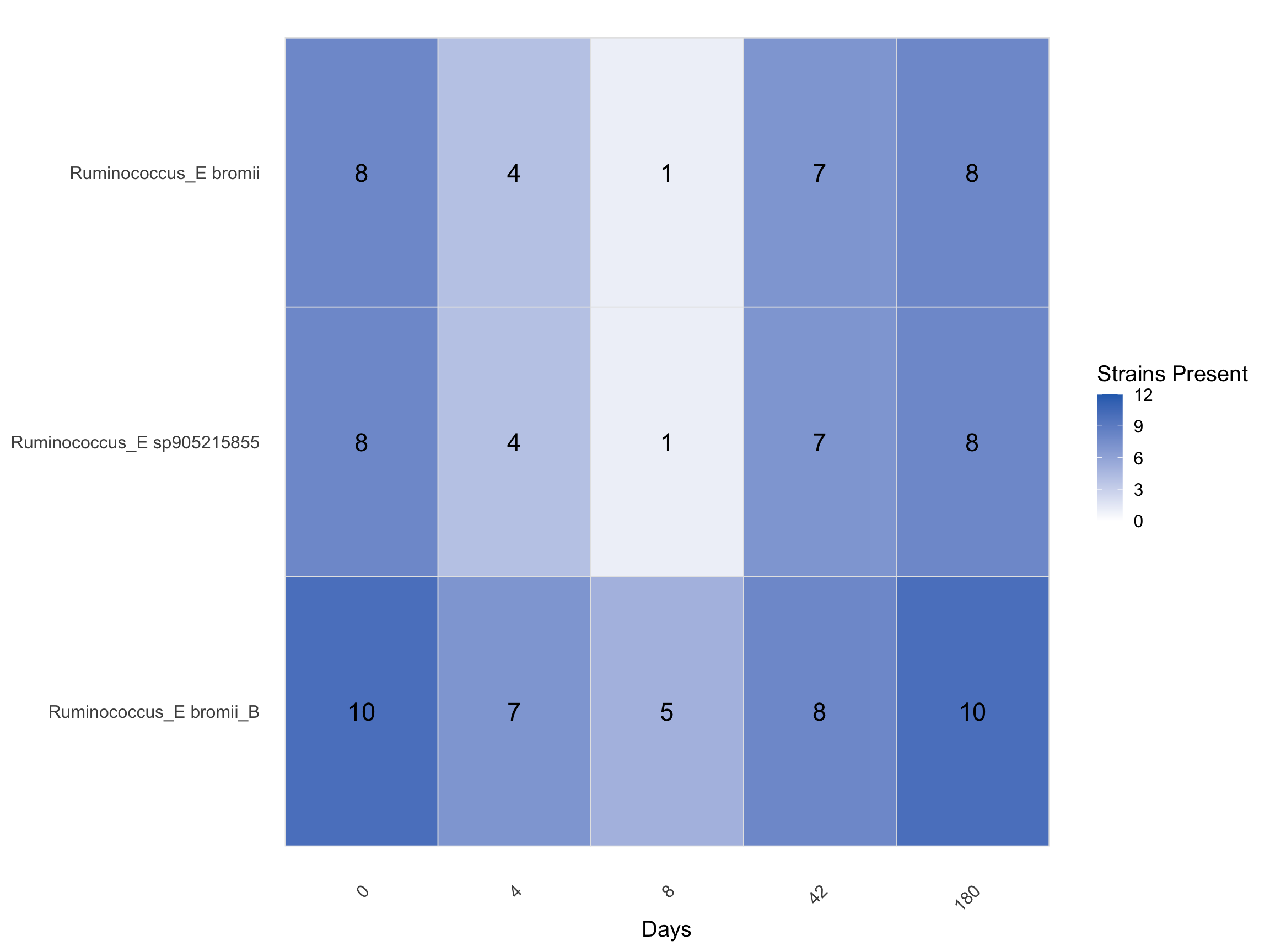
# R. gnavus goes up while other Ruminococci go down and recover
genus_dist("Ruminococcus_B")

genus_dist("Ruminococcus_E")

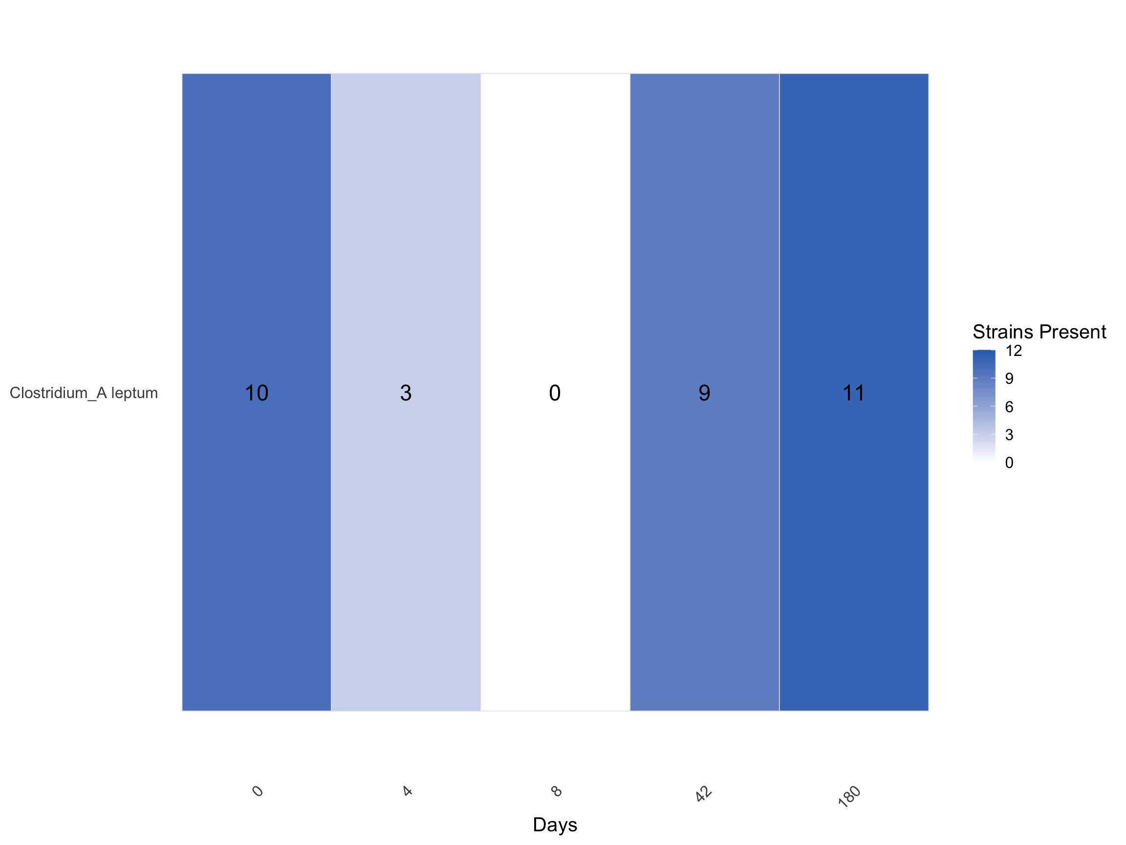
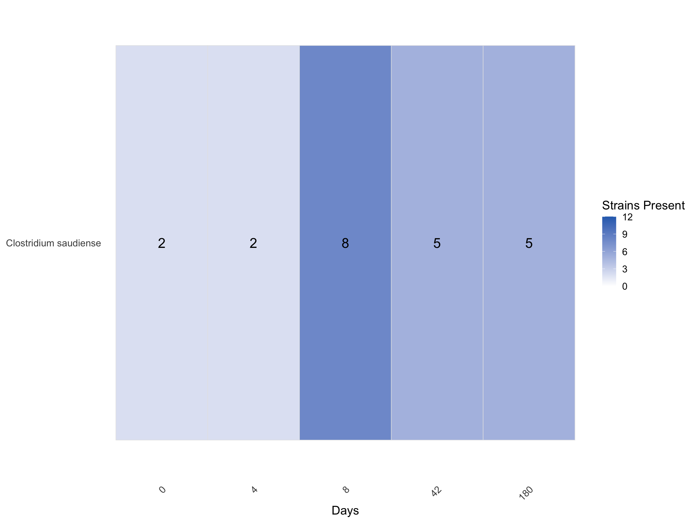
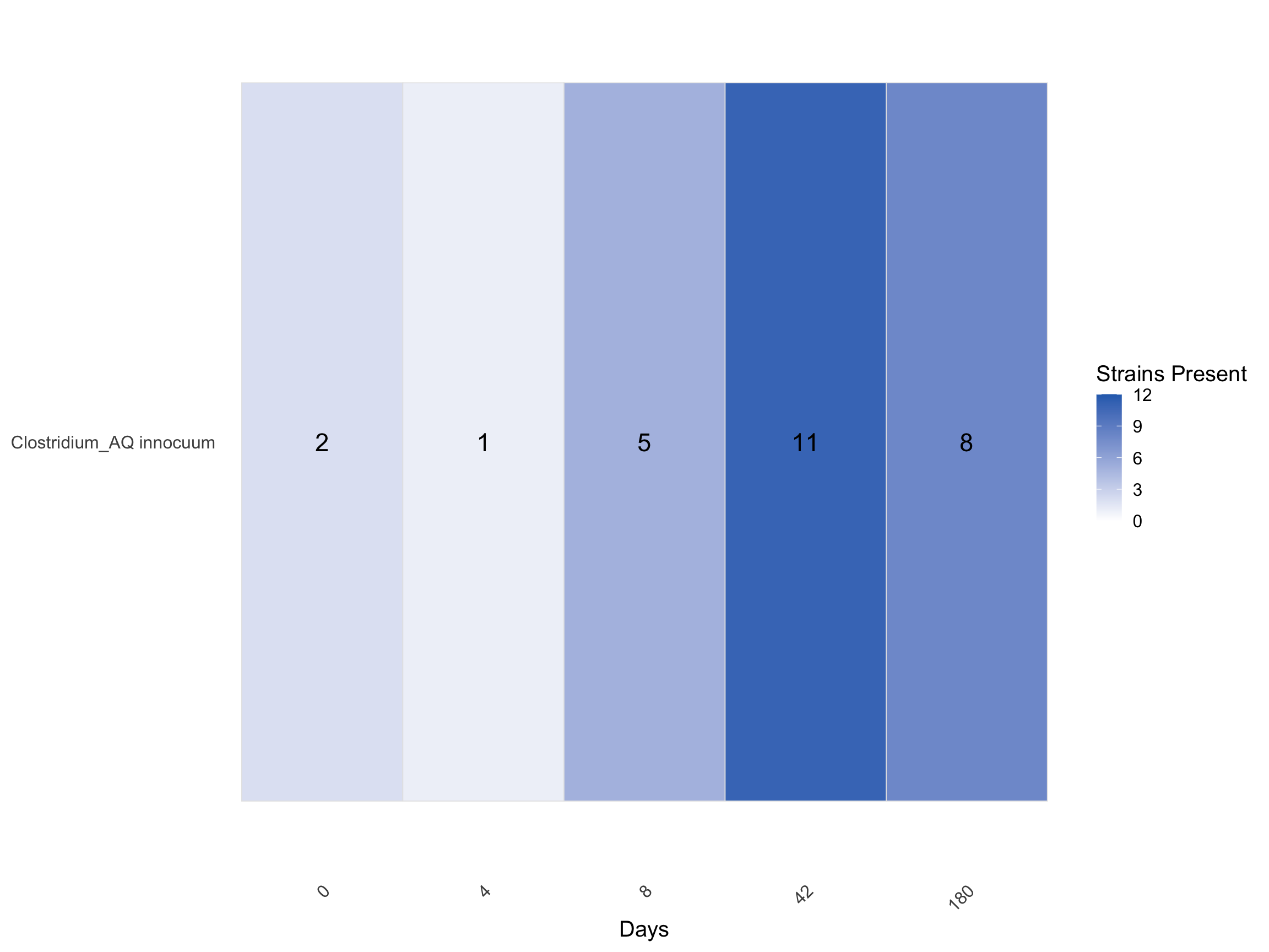
# C leptum (A well known good bacteria) disappears shortly, C innocuum/saudiense (pathobionts) go up. 
# We might be looking at wrong strains here, but the pattern is clear. 
genus_dist("Clostridium_A")

genus_dist("Clostridium")

genus_dist("Clostridium_AQ")

Check for abundance signal

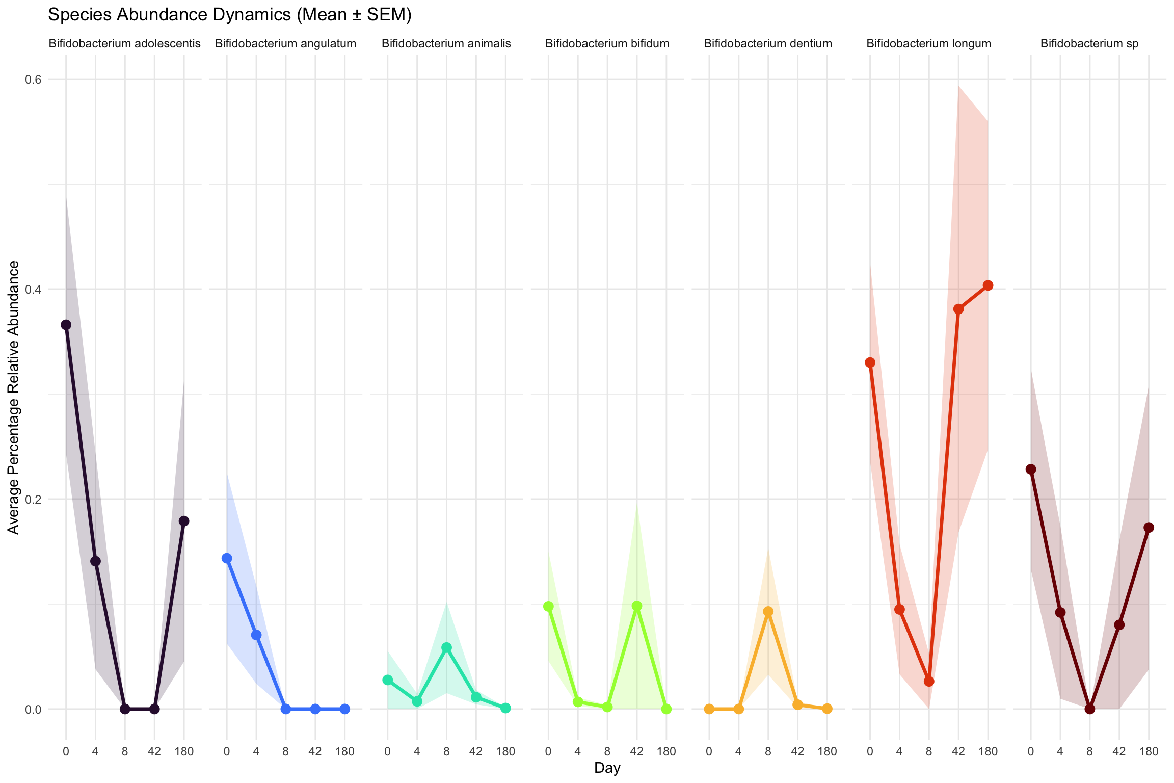
plot_avg_abundance = function(asy_mx, meta){
  # 1. Pivot and Join (as before)
  combined_data <- asy_mx %>% 
    as.data.frame() %>%
    tibble::rownames_to_column("Species") %>%
    pivot_longer(-Species, names_to = "run_accession", values_to = "Abundance") %>%
    inner_join(meta, by = "run_accession")
  
  # 2. Average across subjects for each Day
  final_summary <- combined_data %>%
    group_by(Species, days) %>%
    summarise(
      avg_abundance = mean(Abundance, na.rm = TRUE),
      sem = sd(Abundance, na.rm = TRUE) / sqrt(n()),
      n_subjects = n_distinct(subject), # Confirming data from all 10 subjects
      .groups = "drop"
    ) %>%
    arrange(Species, days)
  
  mapping <- data.frame(
    Species = unique(final_summary$Species), 
    name_fix = strainspy:::clean_contig_names(unique(final_summary$Species))
  )
  
  final_summary <- final_summary %>%
    left_join(mapping, by = "Species")
  
  ggplot(final_summary, aes(x = factor(days), y = avg_abundance, color = name_fix, fill = name_fix, group = name_fix)) +
    # The ribbon now uses the 'fill' aesthetic to match the line color
    geom_ribbon(aes(ymin = avg_abundance - sem, ymax = avg_abundance + sem), alpha = 0.2, color = NA) +
    geom_line(size = 1.2) +
    geom_point(size = 3) +
    facet_wrap(~name_fix, nrow = 1) + # 'free_y' helps see spikes in rare species
    theme_minimal() +
    scale_color_viridis_d(option = "turbo") +
    scale_fill_viridis_d(option = "turbo") + 
    # This removes the legend entirely
    theme(legend.position = "none") +
    labs(
      x = "Day",
      y = "Average Percentage Relative Abundance",
      title = "Species Abundance Dynamics (Mean ± SEM)"
    )
}

# Species level signals
se_p_abud = cleanup(read_sylph("data/palleja_ab_recovery/combined_p_95.tsv", variable = 'Taxonomic_abundance'), meta)

Detected Sylph profile output file.

Retained 371 rows after subject-aware filtering

se_p_assay_bifid = as.matrix(SummarizedExperiment::assay(se_p_abud[rownames(se_p_abud)[grep("Bifidobacterium", rownames(se_p_abud))],]))
plot_avg_abundance(se_p_assay_bifid, meta)

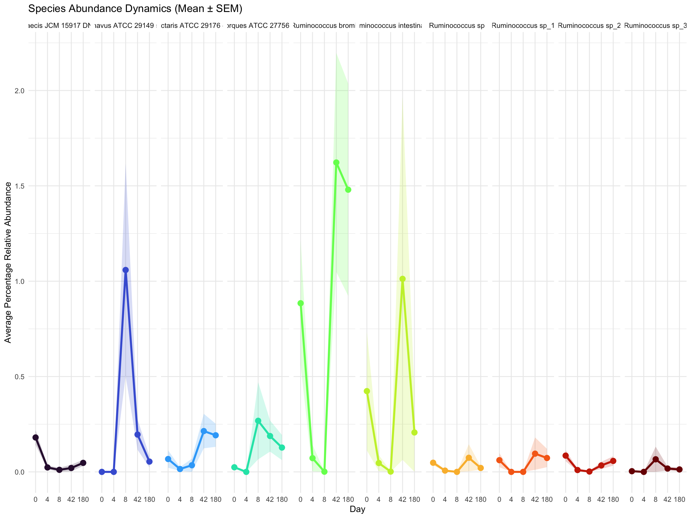
se_p_assay_rum = as.matrix(SummarizedExperiment::assay(se_p_abud[rownames(se_p_abud)[grep("Ruminococcus", rownames(se_p_abud))],]))
plot_avg_abundance(se_p_assay_rum, meta)

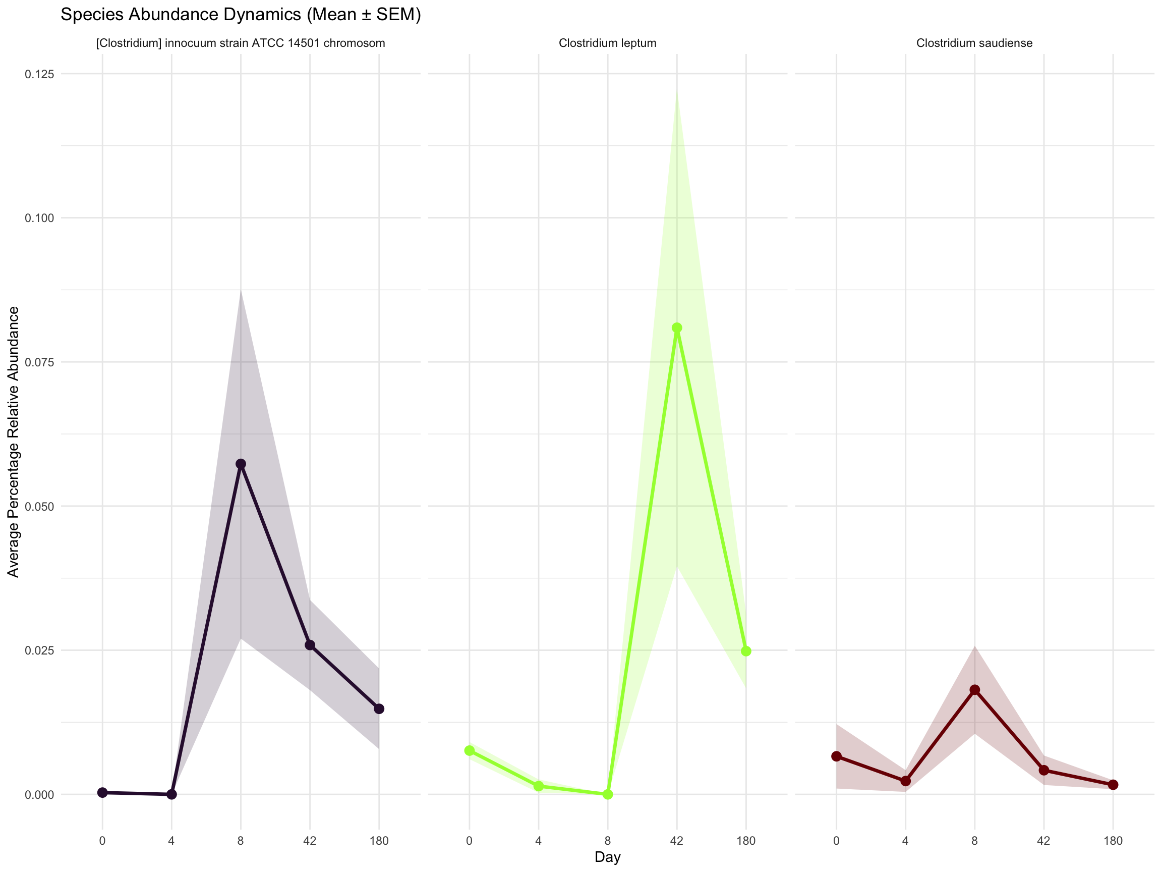
se_p_assay_clos = rbind(as.matrix(SummarizedExperiment::assay(se_p_abud[rownames(se_p_abud)[grep("leptum", rownames(se_p_abud))],])),
                        as.matrix(SummarizedExperiment::assay(se_p_abud[rownames(se_p_abud)[grep("innocuum", rownames(se_p_abud))],])),
                        as.matrix(SummarizedExperiment::assay(se_p_abud[rownames(se_p_abud)[grep("saudiense", rownames(se_p_abud))],])))

plot_avg_abundance(se_p_assay_clos, meta)

Fate of Short-chain fatty acid producing genera

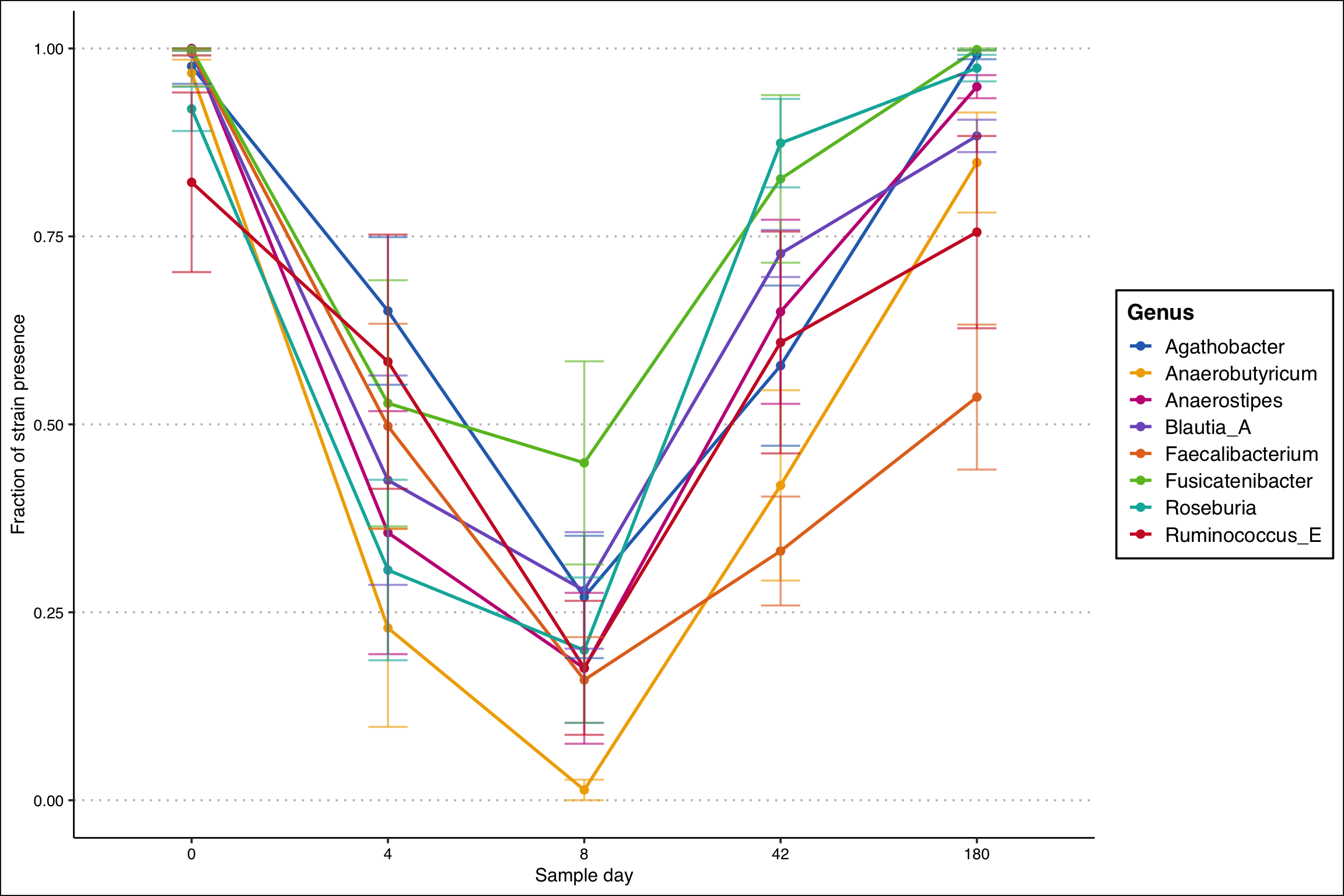
scfa_genera <- c(
  "Faecalibacterium",  # classic butyrate producer
  "Agathobacter",      # Eubacterium rectale group
  "Anaerobutyricum",   # E. hallii group
  "Anaerostipes",      # strong butyrate producer
  "Roseburia",         # hallmark butyrate producer
  "Blautia_A",         # butyrate/acetate producer
  "Fusicatenibacter",  # secondary butyrate producer
  "Ruminococcus_E"     # butyrate producer
)

sfca_non_zeros <- non_zero_counts %>% filter(Genus %in% scfa_genera)
set.seed(25); cols <- ggsci::pal_bmj()(length(unique(sfca_non_zeros$Genus)))

ggplot(sfca_non_zeros, aes(x = days, y = mean_prop_zeros, color = Genus, group = Genus)) +
  geom_line(size = 1) +
  geom_point(size = 2) +
  geom_errorbar(aes(ymin = mean_prop_zeros - se_prop_zeros, ymax = mean_prop_zeros + se_prop_zeros),
                width = 0.2, alpha = 0.6) +
  scale_x_discrete(breaks = sort(unique(sfca_non_zeros$days))) +
  scale_color_manual(values = cols) +
  labs(
    x = "Sample day",
    y = "Fraction of strain presence",
    color = "Genus"
  ) +
  theme(
    legend.position = "right",
    panel.grid.minor = element_blank(),
    plot.title = element_text(face = "bold")
  ) +
  theme_clean(base_size = 14)

Fate of some oppotunistic bacteria

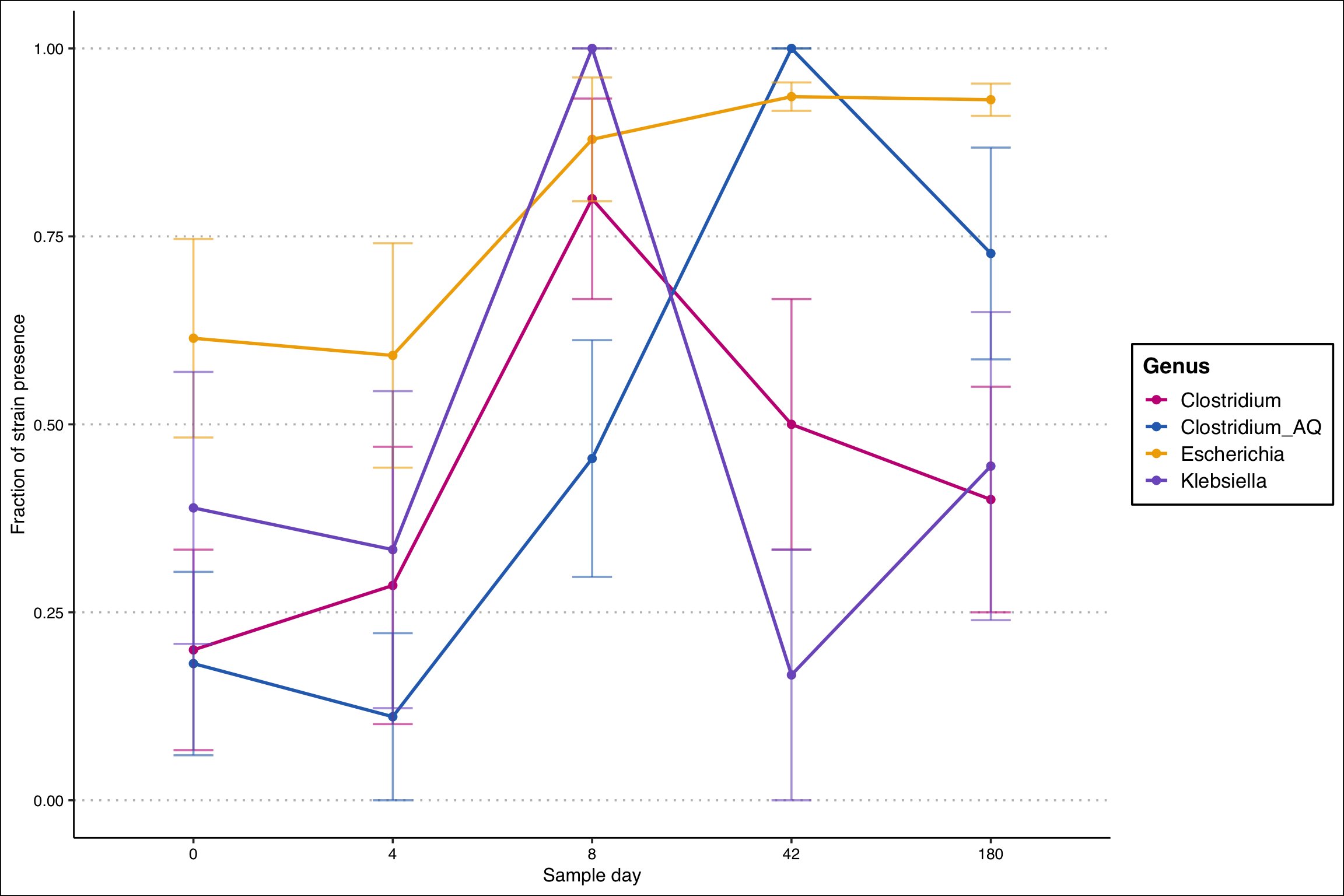
opportunistic_genera <- c(
  "Clostridium",
  "Clostridium_AQ",
  "Klebsiella",
  "Escherichia"       # E. coli and related, classic opportunist
)

opp_non_zeros <- non_zero_counts %>% filter(Genus %in% opportunistic_genera)
set.seed(25); cols <- ggsci::pal_bmj()(length(opportunistic_genera))[sample(length(unique(opp_non_zeros$Genus)))]

ggplot(opp_non_zeros, aes(x = days, y = mean_prop_zeros, color = Genus, group = Genus)) +
  geom_line(size = 1) +
  geom_point(size = 2) +
  geom_errorbar(aes(ymin = mean_prop_zeros - se_prop_zeros, ymax = mean_prop_zeros + se_prop_zeros),
                width = 0.2, alpha = 0.6) +
  scale_x_discrete(breaks = sort(unique(opp_non_zeros$days))) +
  scale_color_manual(values = cols) +
  labs(
    x = "Sample day",
    y = "Fraction of strain presence",
    color = "Genus"
  ) +
  theme_clean(base_size = 14) +
  theme(
    legend.position = "right",
    panel.grid.minor = element_blank(),
    plot.title = element_text(face = "bold")
  )

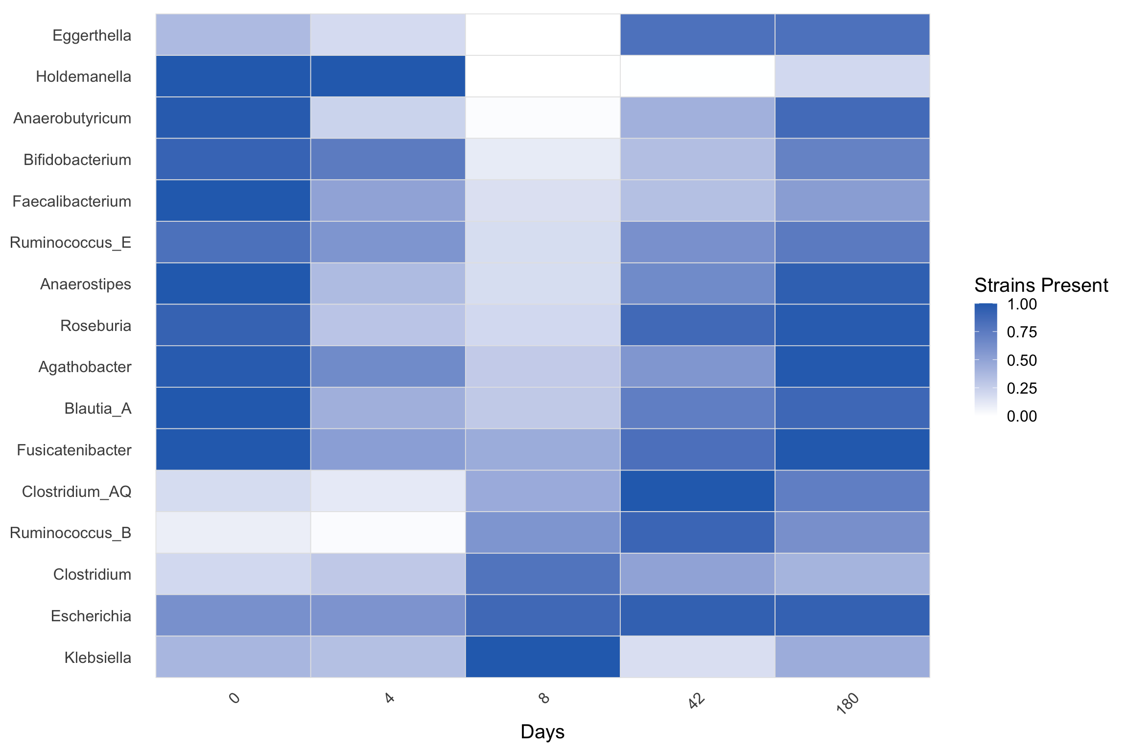
Visualise as a heatmap

Butyrate_genera <- c(
  "Holdemanella",  
  "Anaerostipes",      
  "Roseburia",
  "Faecalibacterium",  # classic butyrate producer
  "Agathobacter",      # Eubacterium rectale group
  "Anaerobutyricum",   # E. hallii group
  "Anaerostipes",      # strong butyrate producer
  "Roseburia",         # hallmark butyrate producer
  "Blautia_A",         # butyrate/acetate producer
  "Fusicatenibacter",  # secondary butyrate producer
  "Ruminococcus_E"    # butyrate producer
  
)

opp_genera = opportunistic_genera <- c(
  "Clostridium",
  "Clostridium_AQ",
  "Klebsiella",
  "Escherichia",
  "Ruminococcus_B",
  "Eggerthella",
  "Bifidobacterium"
)

{
  selected_genera = c(Butyrate_genera, opp_genera)
  
  # get genera counts in the database
  genus_totals <- tax99 %>%
    filter(Genus %in% selected_genera) %>%
    distinct(Genus, Genome) %>%    # unique strain × genus pairs
    group_by(Genus) %>%
    summarize(total_strains = n(), .groups = "drop") %>%
    complete(Genus = selected_genera, fill = list(total_strains = 0))
  
  day_levels <- c("0","4","8","42","180") 
  
  presence_df <- ani_filtered %>%
    filter(Genus %in% selected_genera) %>%
    mutate(days = factor(as.character(days), levels = day_levels),
           present = ANI > 95) %>%
    # count unique contig names per Genus x subject x day where present == TRUE
    group_by(Genus, subject, days) %>%
    summarize(n_strains = n_distinct(Contig_name[present]), .groups = "drop")
  
  
  prop_df <- presence_df %>%
    left_join(genus_totals, by = "Genus") %>%
    mutate(
      # avoid division by zero: if genus has zero total strains, produce NA
      prop_of_genus = if_else(total_strains > 0,
                              n_strains / total_strains,
                              NA_real_)
    )
  
  baseline <- prop_df %>%
    group_by(Genus, subject) %>%
    summarize(
      prop0 = max(prop_of_genus, na.rm = TRUE),   # highest proportion across all days
      .groups = "drop"
    )
  
  prop_df2 <- prop_df %>%
    left_join(baseline, by = c("Genus", "subject"))
  
  prop_df2 <- prop_df2 %>%
    mutate(
      ratio = if_else(!is.na(prop0) & prop0 > 0,
                      prop_of_genus / prop0,
                      NA_real_),      # baseline-0 subjects → NA
      ratio = pmin(ratio, 1)   # cap at 1 so colour means "as present as baseline"
    )
  summary_ratio <- prop_df2 %>%
    group_by(Genus, days) %>%
    summarize(
      mean_ratio = mean(ratio, na.rm = TRUE),
      se_ratio   = sd(ratio, na.rm = TRUE) / sqrt(sum(!is.na(ratio))),
      n_subj     = sum(!is.na(ratio)),
      .groups = "drop"
    ) %>%
    mutate(days = factor(as.character(days), levels = c("0","4","8","42","180")))
  
  # Order genera by effect (optional)
  order_genus <- summary_ratio %>% filter(days == "8") %>% arrange(mean_ratio) %>% pull(Genus) %>% unique()
  summary_ratio <- summary_ratio %>% mutate(Genus = factor(Genus, levels = rev(order_genus)))
  
  # Plot: white -> single colour; limits [0,1]; NA and 0 appear white
  ggplot(summary_ratio, aes(x = days, y = Genus, fill = mean_ratio)) +
    geom_tile(color = "grey90", size = 0.3) +
    scale_fill_gradient(
      low = "white",
      high = cols[2],    # pick a single strong colour
      limits = c(0, 1),
      na.value = "white",
      name = "Strains Present"
    ) +
    labs(x = "Days", y = NULL) +
    theme_minimal(base_size = 15) +
    theme(panel.grid = element_blank(),
          axis.text.x = element_text(angle = 45, hjust = 1))
}

Strain replacement

bact_filt_out = function(genus){
  bact <- top_hits[grep(genus, top_hits$Genus),]
  bact = bact[which(bact$p_adjust < 0.05),]
  bact = bact[order(bact$p_adjust),]
  
  bact_to_pull = unique(bact$Contig_name)
  asy = SummarizedExperiment::assay(se_q)
  asy = as.matrix(asy[unname(sapply(bact_to_pull, function(x) which(x == rownames(asy)))),])
  
  bact_long <- as.data.frame(asy) %>%
    tibble::rownames_to_column("Contig_name") %>%
    pivot_longer(-Contig_name, names_to = "run_accession", values_to = "ANI") %>%
    left_join(meta %>% select(run_accession, subject, days), by = "run_accession") %>%
    mutate(
      Species = top_hits$Species[match(Contig_name, top_hits$Contig_name)],
      Genus   = top_hits$Genus[match(Contig_name, top_hits$Contig_name)]
    )
  
  bact_filtered <- bact_long %>%
    group_by(subject, Contig_name) %>%
    # Keep only those with at least one non-zero ANI for that subject
    filter(any(ANI != 0)) %>%
    ungroup() %>%
    group_by(Contig_name, subject) %>%
    mutate(
      ANI_day0 = ANI[days == 0],        # baseline for that contig+subject
      ANI_relative = ANI - ANI_day0     # drop or gain relative to day0
    ) %>%
    ungroup() %>% 
    filter(abs(ANI_relative)< 10 & abs(ANI_relative) > 1)
  
  return(bact_filtered)
}

bact_filtered = bact_filt_out("Bacteroides")
contigs_subset <-names(sort(table(bact_filtered$Contig_name), decreasing = T))[c(9, 11, 26)]
ct_to_check = contigs_subset

bact_filtered = bact_filt_out("Alistipes")
contigs_subset <-names(sort(table(bact_filtered$Contig_name), decreasing = T))[c(3)]
ct_to_check = c(ct_to_check, contigs_subset)

bact_filtered = bact_filt_out("Veillonella")
contigs_subset <-names(sort(table(bact_filtered$Contig_name), decreasing = T))[c(8,2)]
ct_to_check = c(ct_to_check, contigs_subset)

bact_filtered = bact_filt_out("Prevotella")
contigs_subset <-names(sort(table(bact_filtered$Contig_name), decreasing = T))[c(2)]
ct_to_check = c(ct_to_check, contigs_subset)

bact <- top_hits
bact = bact[which(bact$p_adjust < 0.05),]
bact = bact[order(bact$p_adjust),]

bact_to_pull = unique(bact$Contig_name)
asy = SummarizedExperiment::assay(se_q)
asy = as.matrix(asy[unname(sapply(bact_to_pull, function(x) which(x == rownames(asy)))),])

bact_long <- as.data.frame(asy) %>%
  tibble::rownames_to_column("Contig_name") %>%
  pivot_longer(-Contig_name, names_to = "run_accession", values_to = "ANI") %>%
  left_join(meta %>% select(run_accession, subject, days), by = "run_accession") %>%
  mutate(
    Species = top_hits$Species[match(Contig_name, top_hits$Contig_name)],
    Genus   = top_hits$Genus[match(Contig_name, top_hits$Contig_name)]
  )

bact_filtered <- bact_long %>%
  group_by(subject, Contig_name) %>%
  # Keep only those with at least one non-zero ANI for that subject
  filter(any(ANI != 0)) %>%
  ungroup() %>%
  group_by(Contig_name, subject) %>%
  mutate(
    ANI_day0 = ANI[days == 0],        # baseline for that contig+subject
    ANI_relative = ANI - ANI_day0     # drop or gain relative to day0
  ) %>%
  ungroup() %>% 
  filter(abs(ANI_relative)< 10 & abs(ANI_relative) > 1)
ct_to_check_ = ct_to_check[c(1, 5, 4)]

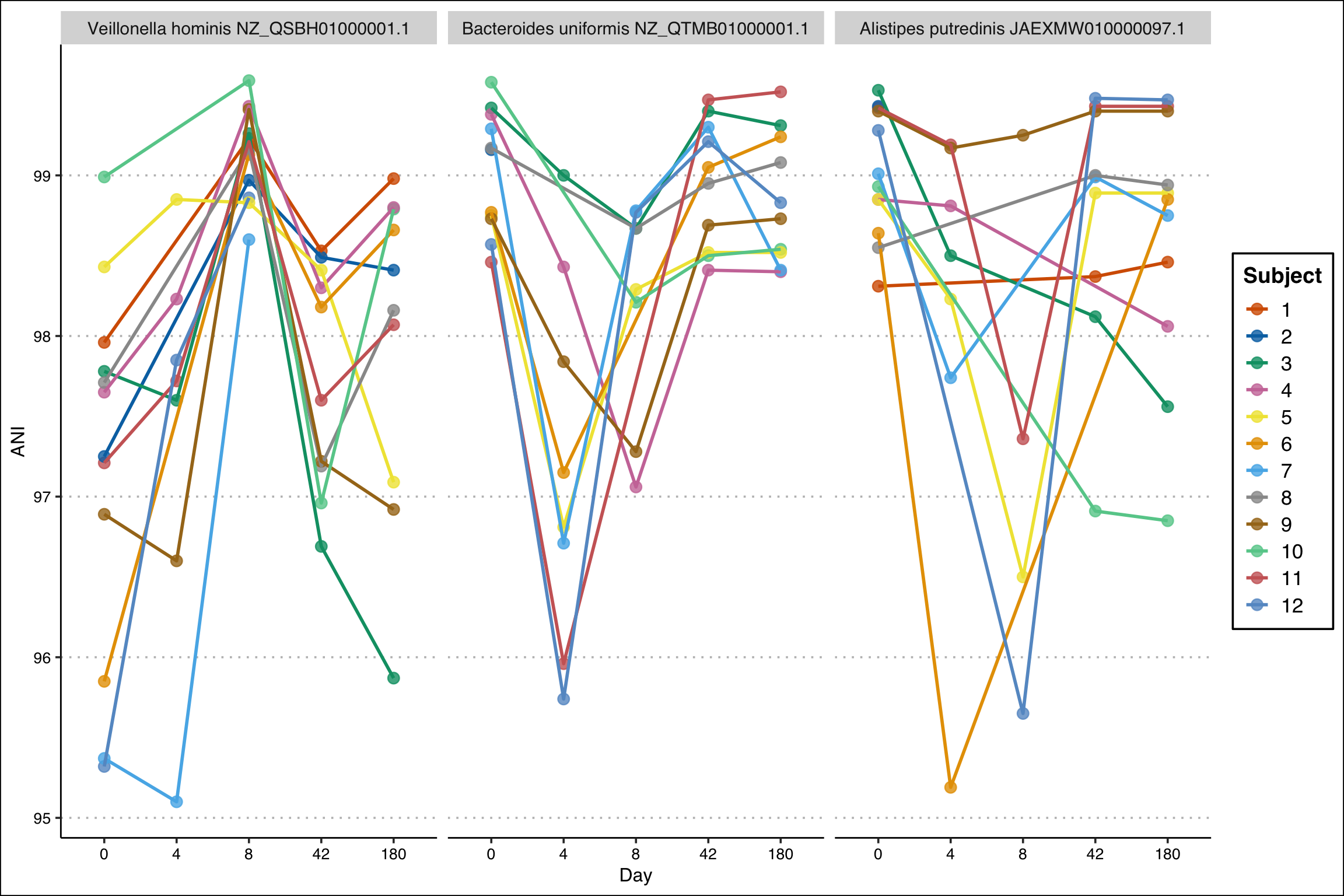
# All hits with very small beta p-values indicate strain replacement, but we also track strain disappearances. Let's try to keep strains that persist 
df_plot <- bact_long %>%
  filter(Contig_name %in% ct_to_check_, ANI > 0)

df_plot$Contig_name = factor(df_plot$Contig_name, levels = ct_to_check_ )

for(i in 1:nrow(df_plot)){
  df_plot$Species[i] = paste(df_plot$Species[i], str_extract(df_plot$Contig_name[i], "^[^ ]+"))
}
df_plot$Species = factor(df_plot$Species, levels = unique(df_plot$Species) )

ggplot(df_plot, aes(x = factor(days), y = ANI, group = subject, color = subject)) +
  geom_point(size = 3, alpha = 0.8) +        # points per subject/day
  geom_line(size = 1) +                      # lines connecting days per subject
  scale_color_manual(values =  c(
    "#D55E00", # reddish-orange  
    "#0072B2", # deep blue  
    "#009E73", # teal/green  
    "#CC79A7", # magenta  
    "#F0E442", # yellow  
    "#E69F00", # orange  
    "#56B4E9", # sky blue  
    "#999999", # gray  
    "#A6761D", # brown  
    "#66CC99", # mint  
    "#CC6666", # muted red  
    "#6699CC"  # muted blue  
  )) +
  facet_wrap(~Species, scales = "free_x") +
  labs(x = "Day", y = "ANI", color = "Subject") +
  theme(axis.text.x = element_text(hjust = 0.5)) +
  theme_clean(base_size = 14)

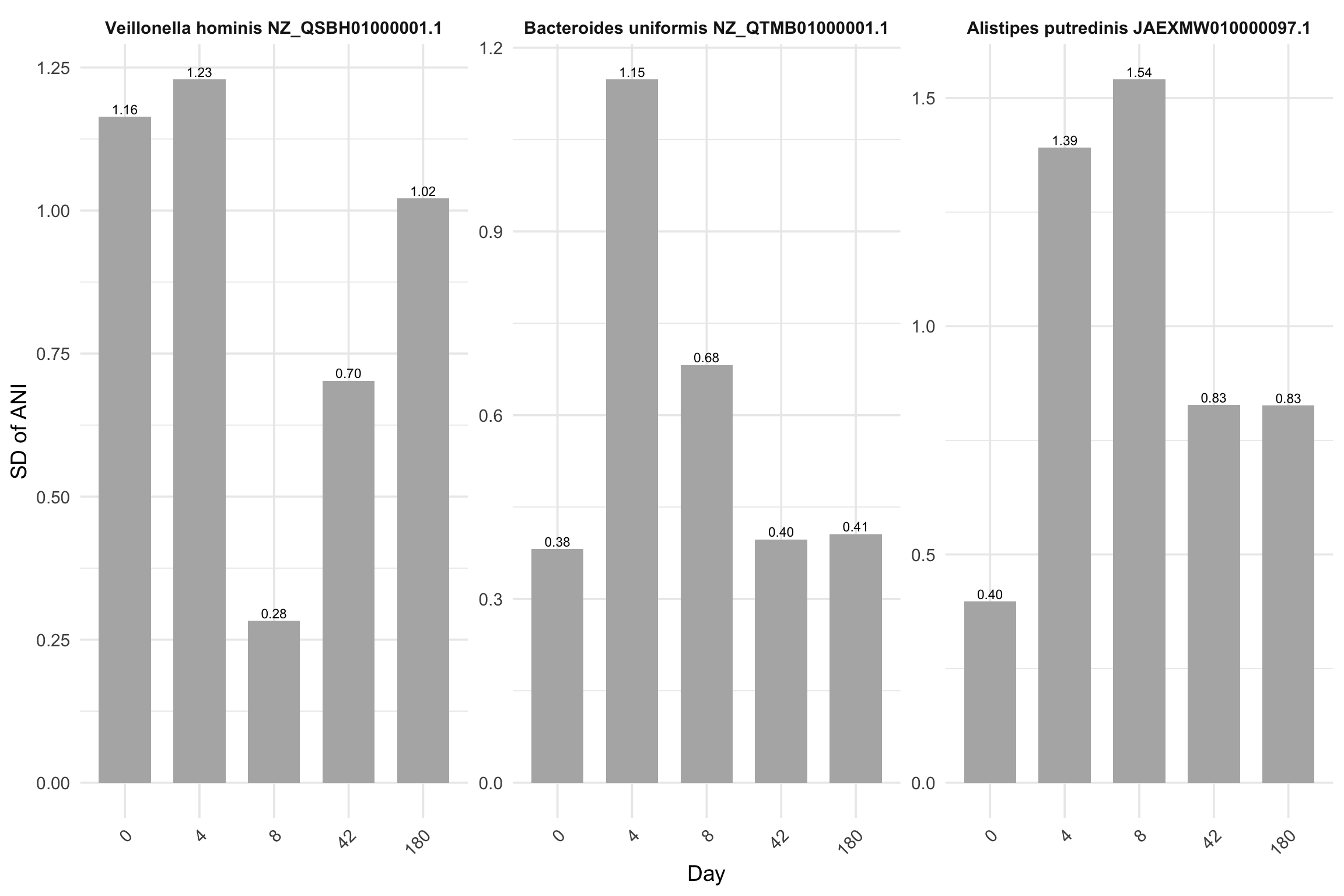
# Strain replacement p-values for these three strains: 4.664351e-12 4.011619e-08 3.600068e-05


df_plot_sd = df_plot %>% group_by(Species,days) %>% summarise(sd_ANI = sd(ANI))

`summarise()` has regrouped the output.
ℹ Summaries were computed grouped by Species and days.
ℹ Output is grouped by Species.
ℹ Use `summarise(.groups = "drop_last")` to silence this message.
ℹ Use `summarise(.by = c(Species, days))` for per-operation grouping
  (`?dplyr::dplyr_by`) instead.

ggplot(df_plot_sd, aes(x = days, y = sd_ANI)) +
  geom_col(width = 0.7, fill = "grey70") +
  
  facet_wrap(~Species, scales = "free_y") +
  
  labs(x = "Day", y = "SD of ANI") +
  
  theme_minimal(base_size = 14) +
  theme(
    strip.text = element_text(face = "bold"),
    axis.text.x = element_text(angle = 45, hjust = 1)
  ) + 
  geom_text(aes(label = sprintf("%.2f", sd_ANI)),
            vjust = -0.3, size = 3)

Paper Figures

## Supplementary abundance
## SFCA_Producers
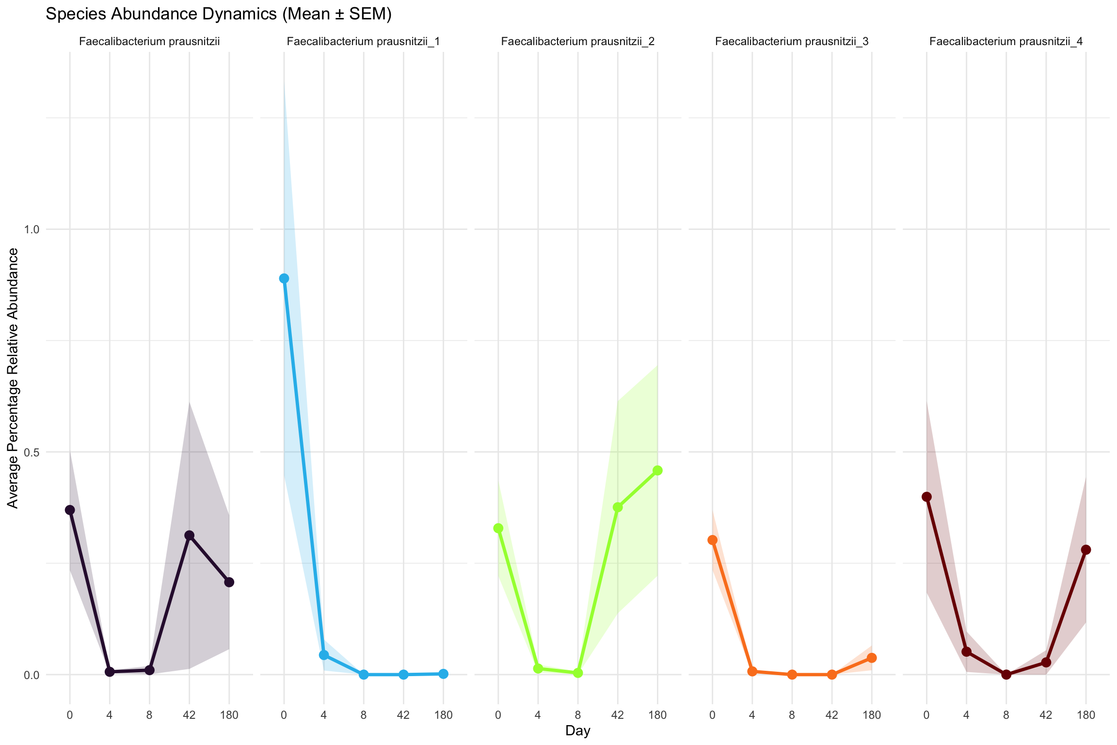
se_p_assay_fp = as.matrix(SummarizedExperiment::assay(se_p_abud[rownames(se_p_abud)[grep("prausnitzii", rownames(se_p_abud))],]))
plot_avg_abundance(se_p_assay_fp, meta)

se_p_assay_bl = as.matrix(SummarizedExperiment::assay(se_p_abud[rownames(se_p_abud)[grep("Bifidobacterium", rownames(se_p_abud))],]))
plot_avg_abundance(se_p_assay_bl, meta)

strain_dist = function(selected_strains){ 
  
  idx_list = sapply(selected_strains, function(x) grep(x, ani_filtered$Contig_name))
  chose_idx = unname(unlist(idx_list))
  
  ani_filtered_ss = ani_filtered[chose_idx,]
  ani_filtered_ss$strain = rep(selected_strains, times = unlist(lapply(idx_list, length)))
  
  
  day_levels <- c("0","4","8","42","180")
  # 12 subjects on all days except 4 (9)
  
  ani_filtered_ss$n_tot_subj = ifelse(ani_filtered_ss$days == 4, 9, 12)
  
  presence_df <- ani_filtered_ss %>%
    mutate(days = factor(as.character(days), levels = day_levels),
           present = ANI > 95) %>%
    # count unique contig names per Genus x subject x day where present == TRUE
    group_by(Species, subject, days) %>%
    summarize(n_strains = n_distinct(Contig_name[present]),
              n_tot_subj = unique(n_tot_subj),
              strain = unique(strain),
              .groups = "drop")
  
  
  summary_ratio <- presence_df %>%
    group_by(days, Species) %>%
    summarize(
      Species = unique(Species),
      mean_ratio = sum(n_strains)/unique(n_tot_subj),
      n_subj = sum(n_strains),
      strain = unique(strain),
      .groups = "drop"
    ) %>%
    mutate(days = factor(as.character(days), levels = c("0","4","8","42","180")))
  
  # Order genera by effect (optional)
  order_species <- summary_ratio %>% filter(days == "8") %>% arrange(mean_ratio) %>% pull(Species) %>% unique()
  summary_ratio <- summary_ratio %>% mutate(Species = factor(Species, levels = rev(order_species)))
  
  # Plot: white -> single colour; limits [0,1]; NA and 0 appear white
  summary_ratio$strain = factor(summary_ratio$strain, levels = rev(selected_strains))
  ggplot(summary_ratio, aes(x = days, y = strain, fill = mean_ratio)) +
    geom_tile(color = "grey90", size = 0.3) +
    geom_text(aes(label = sprintf("%d", n_subj)),
              size = 6) +
    scale_fill_gradient(
      low = "white",
      high = "#2A6EBBFF",    # pick a single strong colour
      limits = c(0, 1),
      na.value = "white",
      name = "Prevalence"
    ) +
    labs(x = "Days", y = NULL) +
    theme_minimal(base_size = 15) +
    theme(panel.grid = element_blank(),
          axis.text.x = element_text(angle = 45, hjust = 1))
}

### ANI presence/absence for following species 
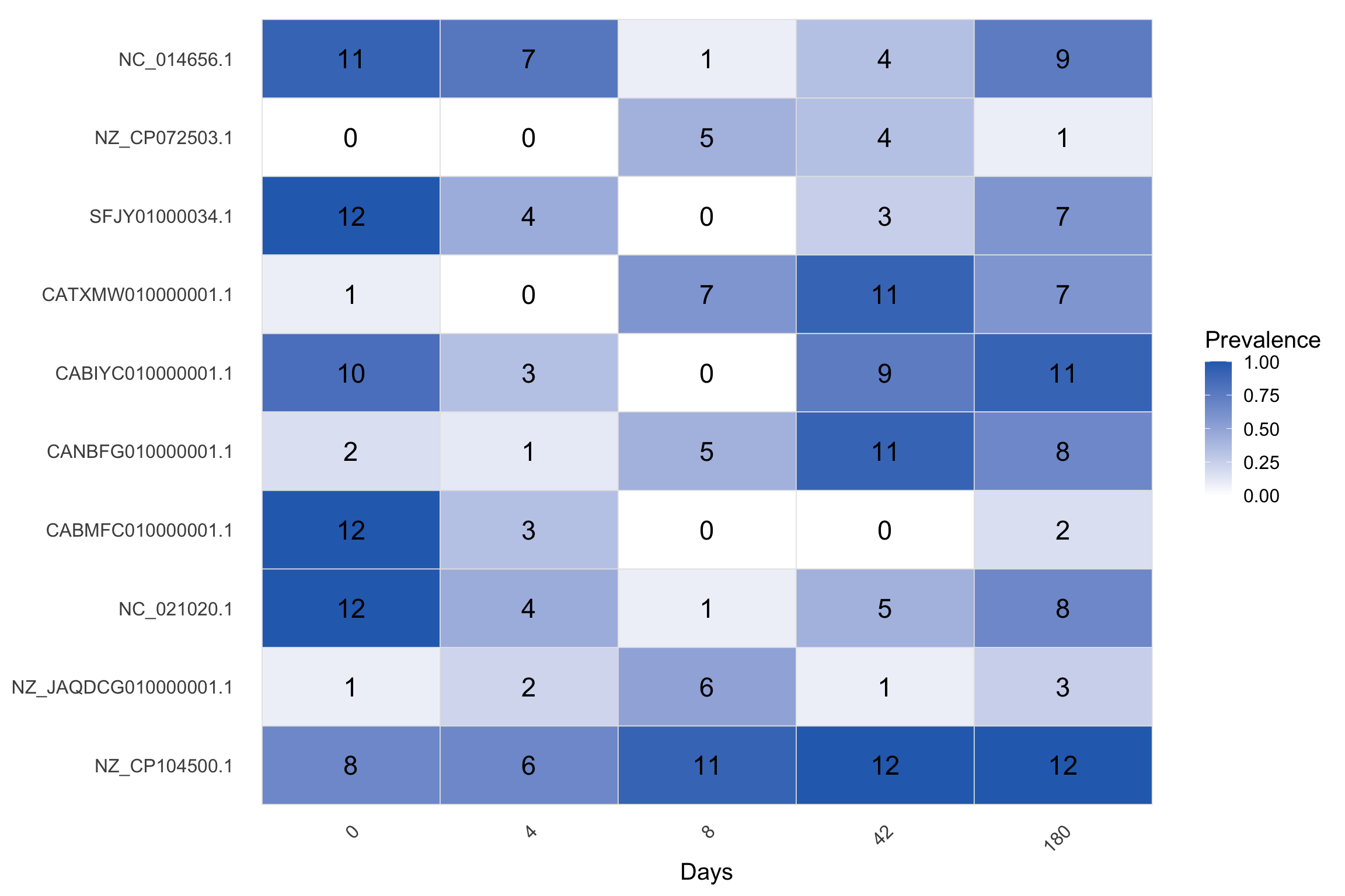
## Competition picture
# Bif longum "NC_014656.1", Bif dentium "NZ_CP072503.1"
# Rum bromii    "SFJY01000034.1", Rum gnavus "CATXMW010000001.1"
# Clos leptum "CABIYC010000001.1", Clos innocuum "CANBFG010000001.1"

## SFCA Picture
# F prausnitzii: CABMFC010000001.1 gone
# F prausnitzii: NC_021020.1 returned

## Oppotunitists
#  Klebs "NZ_JAQDCG010000001.1"
#  E coli "NZ_CP104500.1"

strain_dist(c("NC_014656.1", "NZ_CP072503.1", 
              "SFJY01000034.1", "CATXMW010000001.1",
              "CABIYC010000001.1", "CANBFG010000001.1", 
              "CABMFC010000001.1", "NC_021020.1",
              "NZ_JAQDCG010000001.1",
              "NZ_CP104500.1"))