Analysis of 3414 pooled colorectal cancer metagenomes

Run ZiB analysis in q99 mode

Load dependencies

Load metadata

meta_path <- "./data/segata_pooled_3741/combined_metadata.tsv"
meta <- read.csv(meta_path, sep = '\t') 

# set up contrasts/reference levels
meta$disease = factor(meta$disease, levels = c("Control", "CRC", "Adenoma"))
meta$study = factor(meta$study)
meta$cascon = ifelse(meta$cascon == "Case", "Case", "Control")
meta$cascon = factor(meta$cascon, levels = c("Control", "Case"))
meta$country = factor(meta$country)
meta$sex = factor(meta$sex, levels = c("Female", "Male"))
# let's reset tumour stages
meta$tumour_stage_AJCC[meta$tumour_stage_AJCC == ""] = "NoTumour"
meta$tumour_stage_AJCC[meta$disease == "Adenoma"] = "Adenoma"
meta$tumour_stage_AJCC[meta$tumour_stage_AJCC == "CRC_stage_unlabelled"] = "Unstaged"
meta$tumour_stage_AJCC = factor(meta$tumour_stage_AJCC, levels = c("NoTumour", "Adenoma", "0", "I", "II", "III", "IV", "Unstaged"))

meta$tumour_location[meta$disease == "Control"] = "NoTumour"
meta$tumour_location[meta$disease == "Adenoma"] = "Adenoma"
meta$tumour_location = factor(meta$tumour_location, levels = c("NoTumour", "Adenoma", "transverse", "left_sided", "right_sided", "multiple_sites", "nd"))

Load sylph outputs

sy <- read_sylph("./data/segata_pooled_3741/combined_q_99.tsv.gz") # q99)

Detected Sylph query output file.

sy <- filter_by_presence(sy, min_nonzero = 342) # filter at 10%

Retained 20476 rows after filtering

# annoying renames to match meta V sylph file
colnames(sy) <- gsub("_1", "", colnames(sy))
colnames(sy) <- gsub("_merged", "", colnames(sy))
colData(sy)$Sample_file <- gsub("_1", "", basename(colData(sy)$Sample_file))
colData(sy)$Sample_file <- gsub("_merged", "", colnames(sy))

dim(sy)

[1] 20476  3414

# Checks before merging metadata
all(colnames(sy) %in% meta$run_accession)

[1] TRUE

all(meta$run_accession %in% colnames(sy))

[1] TRUE

sy = modify_metadata(sy, meta)

Fit the model

design <- as.formula("~ disease + age + sex + BMI + (1 | study)")

save_path <- "output_rds/CRC_zib_q_99_ebp.rds"
# Run with ebp - this looks a bit less noisy
if(file.exists(save_path)){
  ZB_fit <- readRDS(save_path)
} else {
  ebp = compute_eb_priors(sy, strainspy:::nobars_(design), nthreads = parallel::detectCores(),low_cutoff = 0, high_cutoff = Inf)
  ZB_fit <- glmZiBFit(sy, design, MAP_prior = ebp, nthreads = parallel::detectCores())
  saveRDS(ZB_fit, save_path)
}

Visualise Outputs

Load GTDB taxonomy

taxonomy <- read_taxonomy("data/TAXONOMY/sylph_DB_taxonomy_99.tsv")

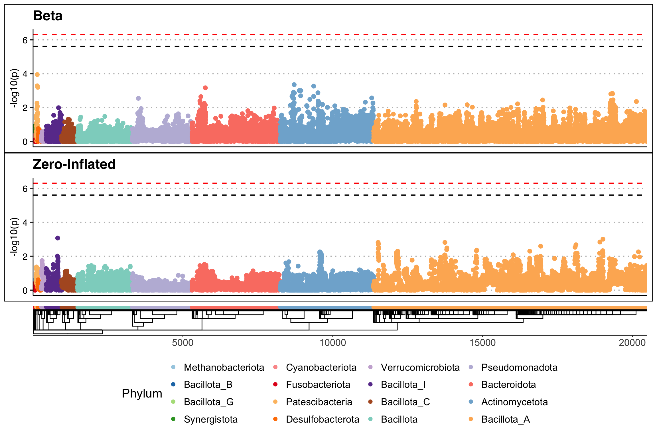
Manhattan and Volcano plots

Control vs. Adenoma

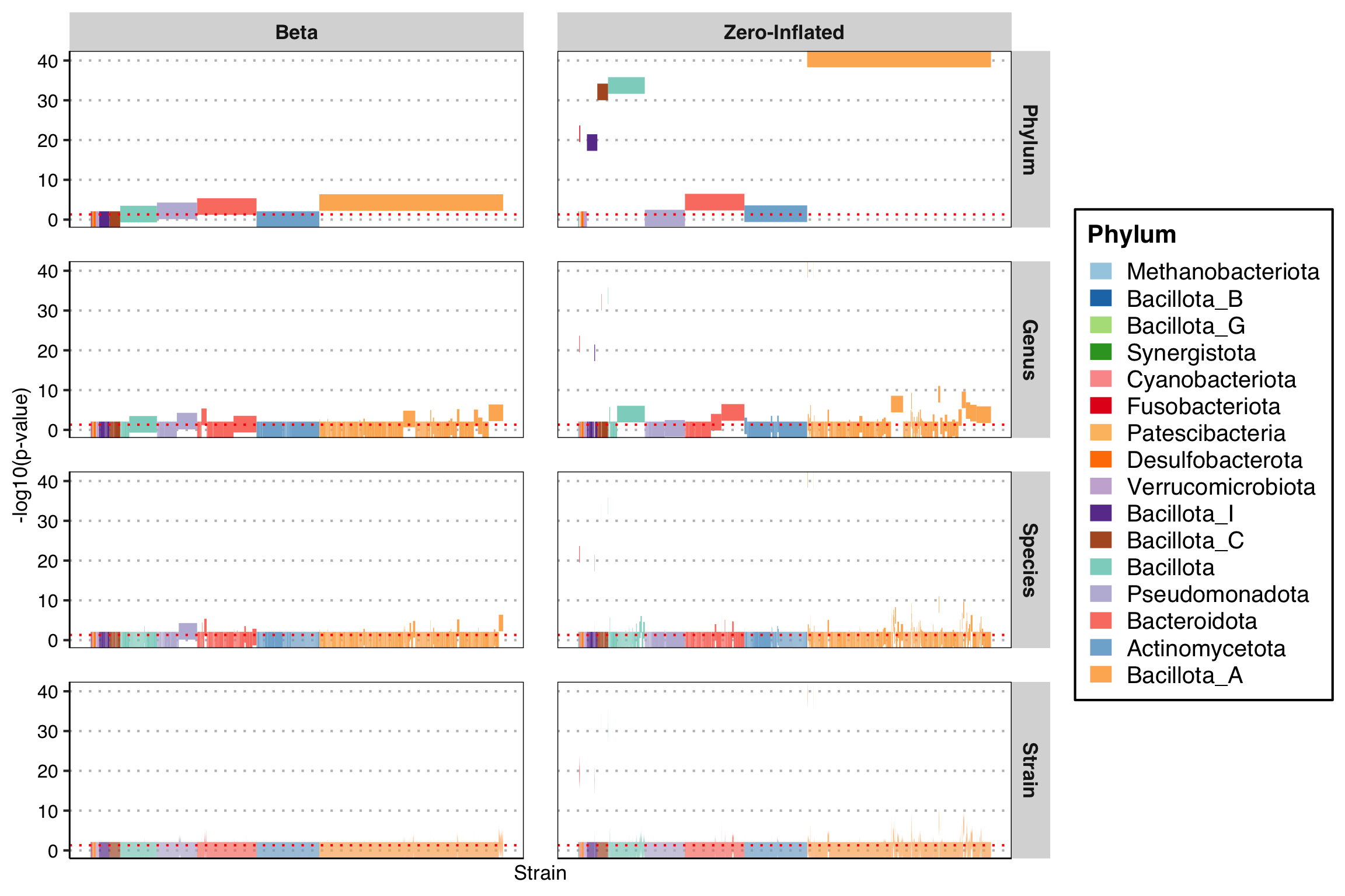
plot_manhattan(ZB_fit, taxonomy = taxonomy, aggregate_by_taxa = T, coef = 3)

! # Invaild edge matrix for <phylo>. A <tbl_df> is returned.
! # Invaild edge matrix for <phylo>. A <tbl_df> is returned.
! # Invaild edge matrix for <phylo>. A <tbl_df> is returned.
! # Invaild edge matrix for <phylo>. A <tbl_df> is returned.

Warning: Using `size` aesthetic for lines was deprecated in ggplot2 3.4.0.
ℹ Please use `linewidth` instead.
ℹ The deprecated feature was likely used in the strainspy package.
  Please report the issue at <https://github.com/gtonkinhill/strainspy/issues>.

plot_manhattan(ZB_fit, taxonomy = taxonomy, aggregate_by_taxa = F, coef = 3)

! # Invaild edge matrix for <phylo>. A <tbl_df> is returned.
! # Invaild edge matrix for <phylo>. A <tbl_df> is returned.
! # Invaild edge matrix for <phylo>. A <tbl_df> is returned.
! # Invaild edge matrix for <phylo>. A <tbl_df> is returned.
! # Invaild edge matrix for <phylo>. A <tbl_df> is returned.
! # Invaild edge matrix for <phylo>. A <tbl_df> is returned.

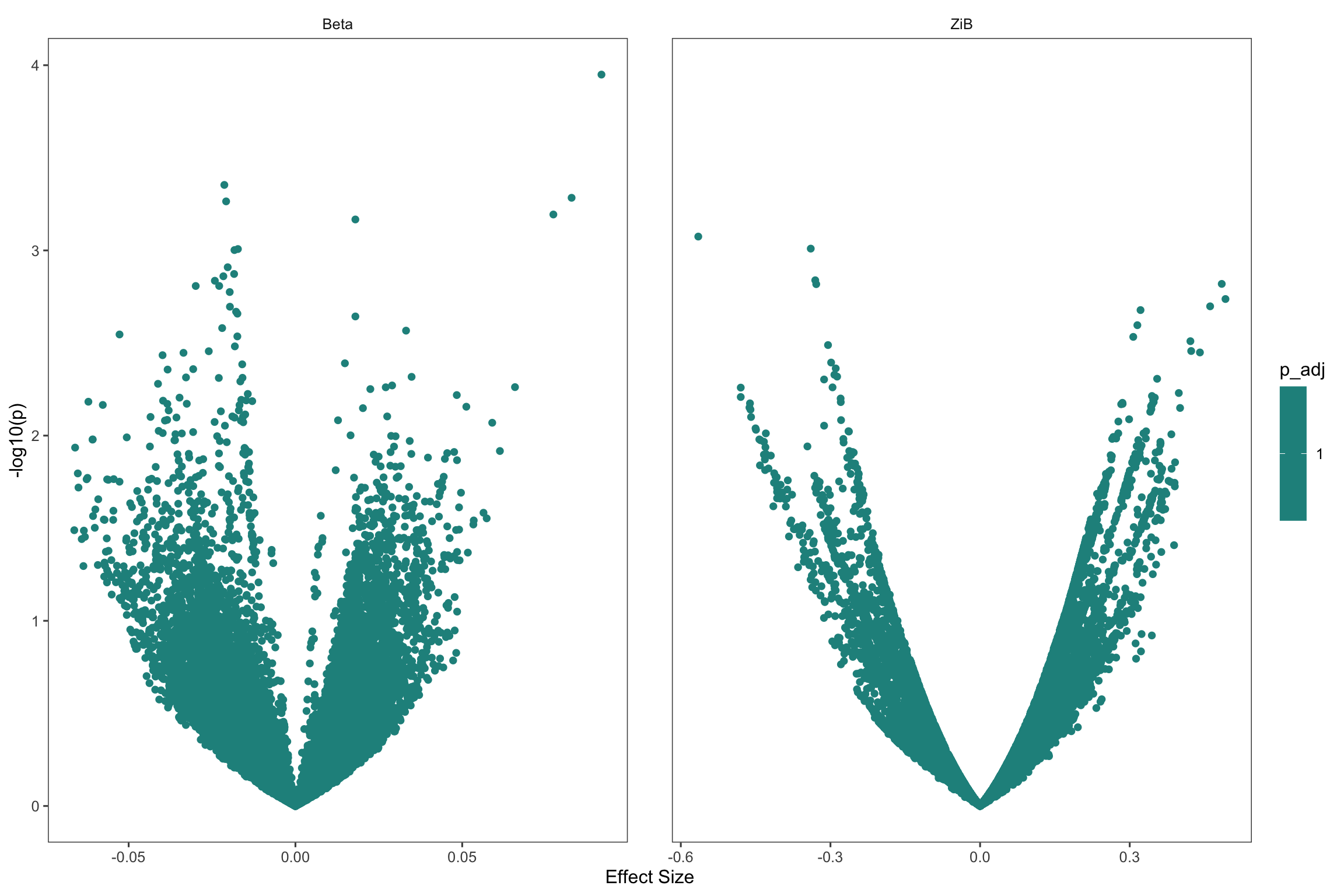
plot_volcano(ZB_fit, coef = 3)

Found 20476 tophits for diseaseAdenoma at alpha = 1 using holm 

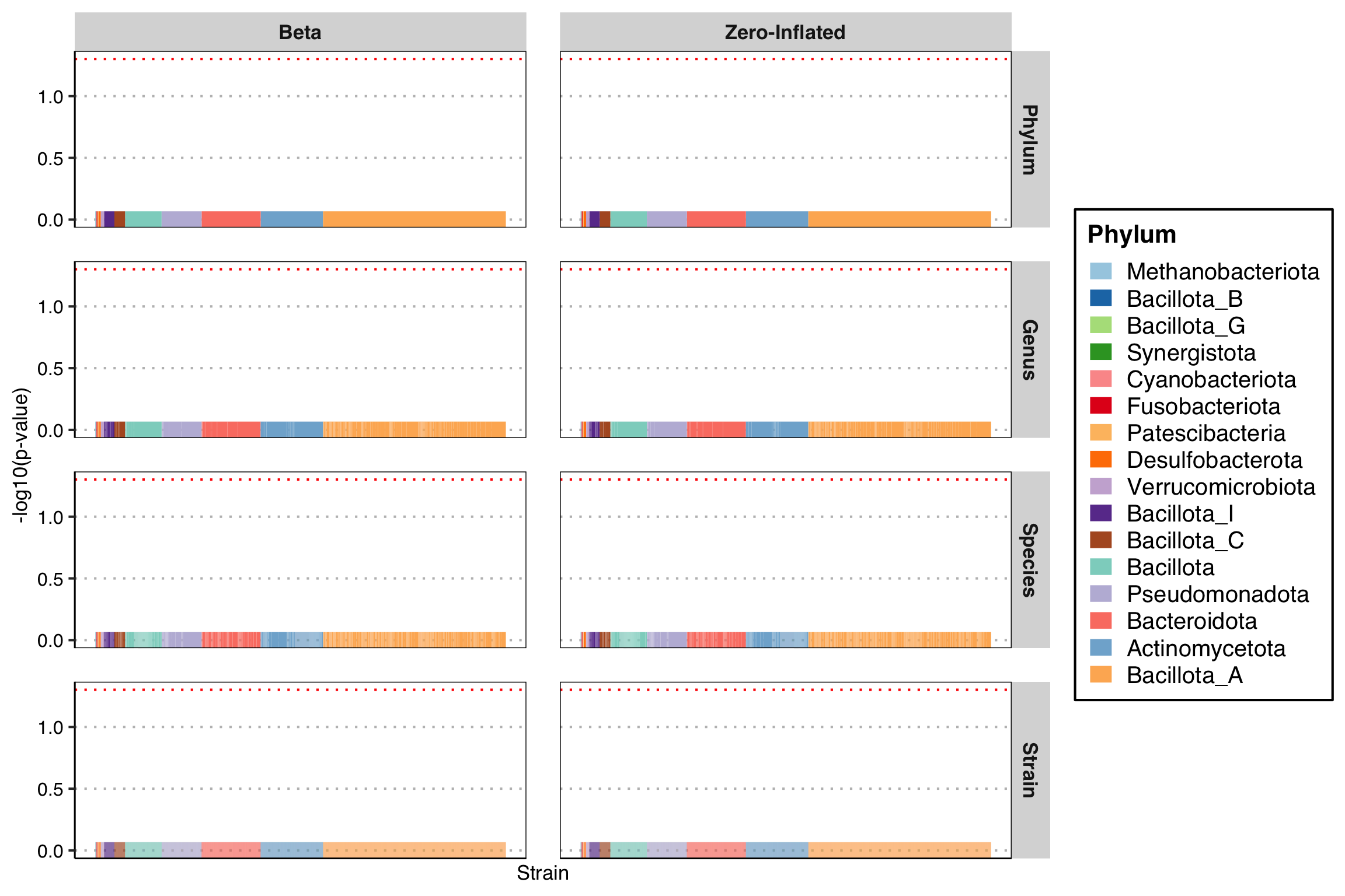
No real signal detected. This agrees with the original paper.

Control vs. CRC

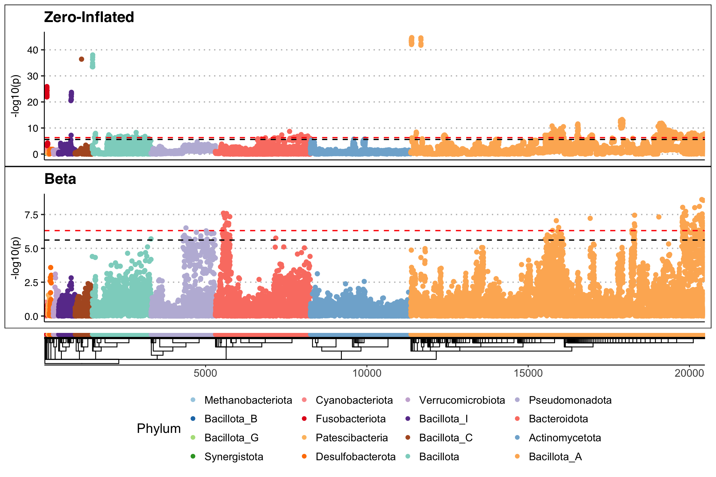
plot_manhattan(ZB_fit, taxonomy = taxonomy, aggregate_by_taxa = T, coef = 2) 

! # Invaild edge matrix for <phylo>. A <tbl_df> is returned.
! # Invaild edge matrix for <phylo>. A <tbl_df> is returned.
! # Invaild edge matrix for <phylo>. A <tbl_df> is returned.
! # Invaild edge matrix for <phylo>. A <tbl_df> is returned.

plot_manhattan(ZB_fit, taxonomy = taxonomy, aggregate_by_taxa = F, coef = 2) 

! # Invaild edge matrix for <phylo>. A <tbl_df> is returned.
! # Invaild edge matrix for <phylo>. A <tbl_df> is returned.
! # Invaild edge matrix for <phylo>. A <tbl_df> is returned.
! # Invaild edge matrix for <phylo>. A <tbl_df> is returned.
! # Invaild edge matrix for <phylo>. A <tbl_df> is returned.
! # Invaild edge matrix for <phylo>. A <tbl_df> is returned.

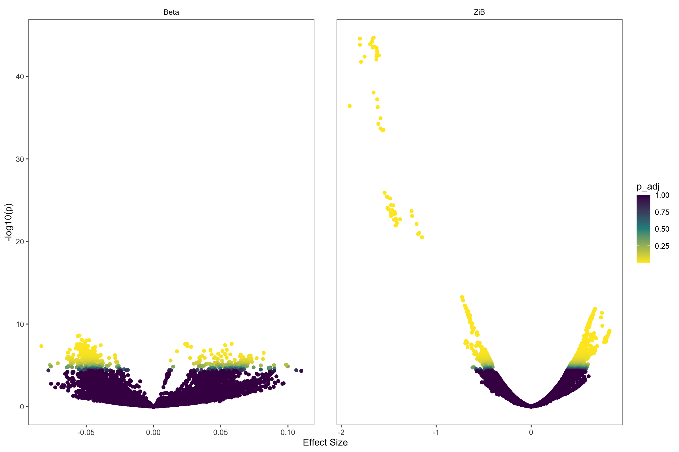
plot_volcano(ZB_fit, coef = 2)

Found 20476 tophits for diseaseCRC at alpha = 1 using holm 

Looks like there are many hits.

Summarise and inspect

Build a summary from top hits

th = comp_ani_diff_and_posthoc_test(se = sy, fit = ZB_fit, th = top_hits(ZB_fit, coef = 2), progress = FALSE)

Found 974 tophits for diseaseCRC at alpha = 0.05 using holm 

th = th[is.na(th$Comment), ]
th = strainspy:::add_tax2tophits(th, taxonomy)

# Remove the weakly separated beta hits (somewhat arbitrary 5.75% - somewhat arbitrary, but no way around manual checks to see separations
rmidx = which(abs(th$ANI_Difference) < 0.0575)
if(length(rmidx) > 0) th = th[-rmidx, ]

# Signals detected from 70 species
length(sort(table(th$Species), decreasing = T))

[1] 70

# Ask chatGPT for a nice summary table
summary_tbl <- th %>%
  filter(!is.na(Species)) %>%
  group_by(Species) %>%
  summarise(
    N_hits = n(),
    
    Top_adj_p_beta  = min(p_adjust, na.rm = TRUE),
    Top_coef_beta   = coefficient[which.min(p_adjust)],
    Top_se_beta     = std_error[which.min(p_adjust)],
    Top_contig_beta = Contig_name[which.min(p_adjust)],
    
    Top_adj_p_ZI    = min(zi_p_adjust, na.rm = TRUE),
    Top_coef_ZI     = zi_coefficient[which.min(zi_p_adjust)],
    Top_se_ZI       = zi_std_error[which.min(zi_p_adjust)],
    Top_contig_ZI   = Contig_name[which.min(zi_p_adjust)],
    
    .groups = "drop"
  ) %>%
  mutate(
    Min_adj_p = pmin(Top_adj_p_beta, Top_adj_p_ZI, na.rm = TRUE),
    Dominant_component = ifelse(Top_adj_p_beta < Top_adj_p_ZI, "Beta", "ZI"),
    Dominant_contig    = ifelse(Dominant_component == "Beta", Top_contig_beta, Top_contig_ZI),
    Dominant_coef      = ifelse(Dominant_component == "Beta", Top_coef_beta, Top_coef_ZI),
    Dominant_se        = ifelse(Dominant_component == "Beta", Top_se_beta, Top_se_ZI)
  ) %>%
  select(Species, N_hits, Dominant_component, Min_adj_p, Dominant_coef, Dominant_se, Dominant_contig) %>%
  arrange(Min_adj_p)

# Write as tsv for manual perusal
# write.table(summary_tbl, "output_tables/CRC_Z99_ebp_summary.tsv", sep = '\t', col.names = T, row.names = F, quote = F)

ZI component hits

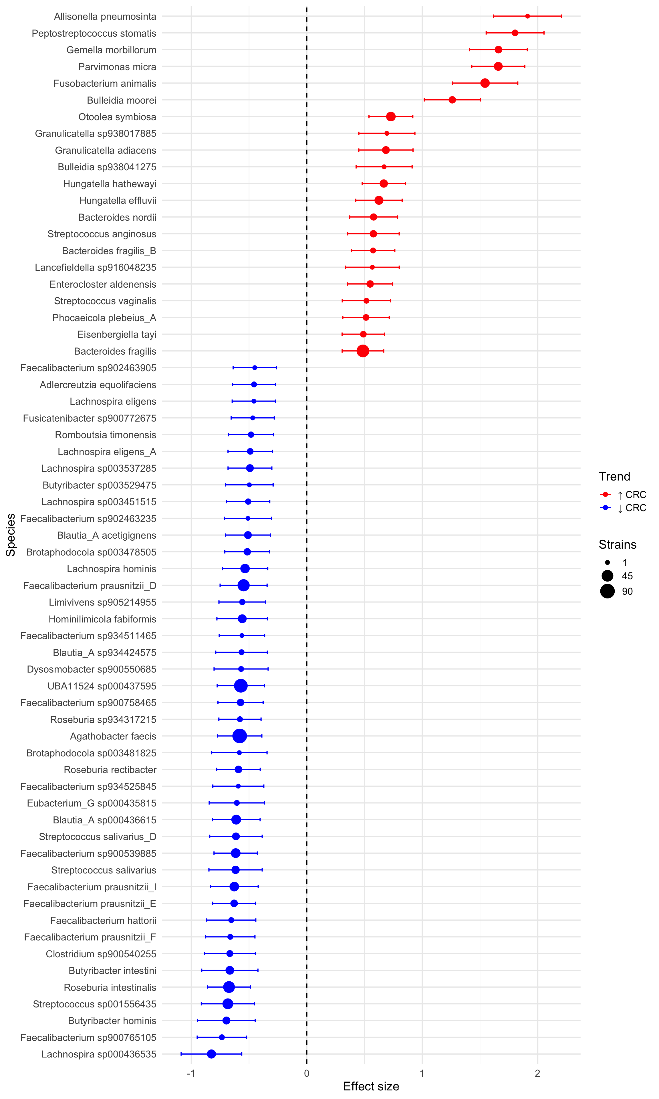
When the Dominant_component is ZI, negative and positive Dominant_coef indicates presence and absence in CRC compared to control.

Visualise this in a forest plot

zi_summary <- summary_tbl %>%
  filter(Dominant_component == "ZI") %>%
  arrange(Min_adj_p) %>%
  mutate(
    # Confidence interval before flipping
    CI_low = Dominant_coef - 1.96 * Dominant_se,
    CI_high = Dominant_coef + 1.96 * Dominant_se,
    
    # Flip effect size and CI
    Dominant_coef = -Dominant_coef,
    CI_low = -CI_low,
    CI_high = -CI_high,
    
    # Trend annotation
    Trend = ifelse(Dominant_coef > 0, "\u2191 CRC", "\u2193 CRC")
  ) %>%
  arrange(Trend, desc(Dominant_coef)) %>%
  mutate(Species = factor(Species, levels = rev(unique(Species))))

ggplot(zi_summary, aes(x = Dominant_coef, y = Species, color = Trend)) +
  geom_point(aes(size = N_hits)) +
  geom_errorbarh(aes(xmin = CI_low, xmax = CI_high), width = 0.2) +
  geom_vline(xintercept = 0, linetype = "dashed") +
  scale_color_manual(values = c("\u2191 CRC" = "red", "\u2193 CRC" = "blue")) +
  scale_size_continuous(
    name = "Strains",
    range = c(2, 8),  # tweak for your figure aesthetics
    breaks = c(1, 45, 90),
    labels = c("1", "45", "90"),
    guide = guide_legend(override.aes = list(linetype = 0))  # remove lines from legend
  ) +
  labs(
    x = "Effect size",
    y = "Species",
    color = "Trend"
  ) +
  theme_minimal(base_size = 16)

Warning: `geom_errorbarh()` was deprecated in ggplot2 4.0.0.
ℹ Please use the `orientation` argument of `geom_errorbar()` instead.

Beta component hits

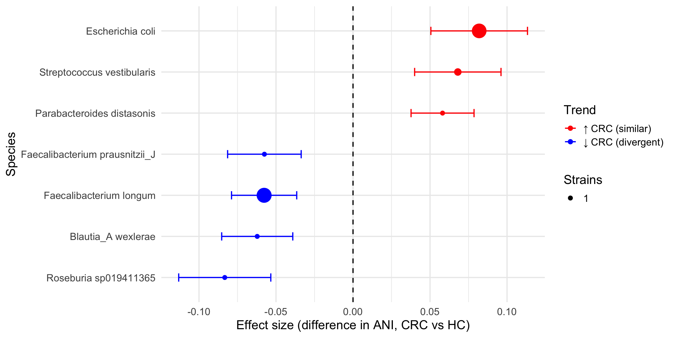
When the Dominant_component is Beta, negative and positive Dominant_coef indicates lower and higher cANI in CRC compared to control, reflecting similarity of the strain to the reference. Higher estimates imply possibly larger strain differences in CRC compared to controls.

beta_summary <- summary_tbl %>%
  filter(Dominant_component == "Beta") %>%
  arrange(Min_adj_p) %>%
  mutate(
    CI_low = Dominant_coef - 1.96 * Dominant_se,
    CI_high = Dominant_coef + 1.96 * Dominant_se,
    Trend = ifelse(Dominant_coef > 0, "\u2191 CRC (similar)", "\u2193 CRC (divergent)"),
    Species = factor(Species, levels = rev(unique(Species)))
  ) %>%
  arrange(desc(Dominant_coef)) %>%
  mutate(Species = factor(Species, levels = rev(unique(Species))))

ggplot(beta_summary, aes(x = Dominant_coef, y = Species, color = Trend)) +
  geom_point(aes(size = N_hits)) +
  geom_errorbarh(aes(xmin = CI_low, xmax = CI_high), width = 0.2) +
  geom_vline(xintercept = 0, linetype = "dashed") +
  scale_color_manual(values = c("\u2191 CRC (similar)" = "red",
                                "\u2193 CRC (divergent)" = "blue")) +
  scale_size_continuous(
    name = "Strains",
    range = c(2, 8),
    breaks = c(1, 60, 120),
    labels = c("1", "60", "120")
  ) +
  labs(
    x = "Effect size (difference in ANI, CRC vs HC)",
    y = "Species",
    color = "Trend"
  ) +
  theme_minimal(base_size = 16)

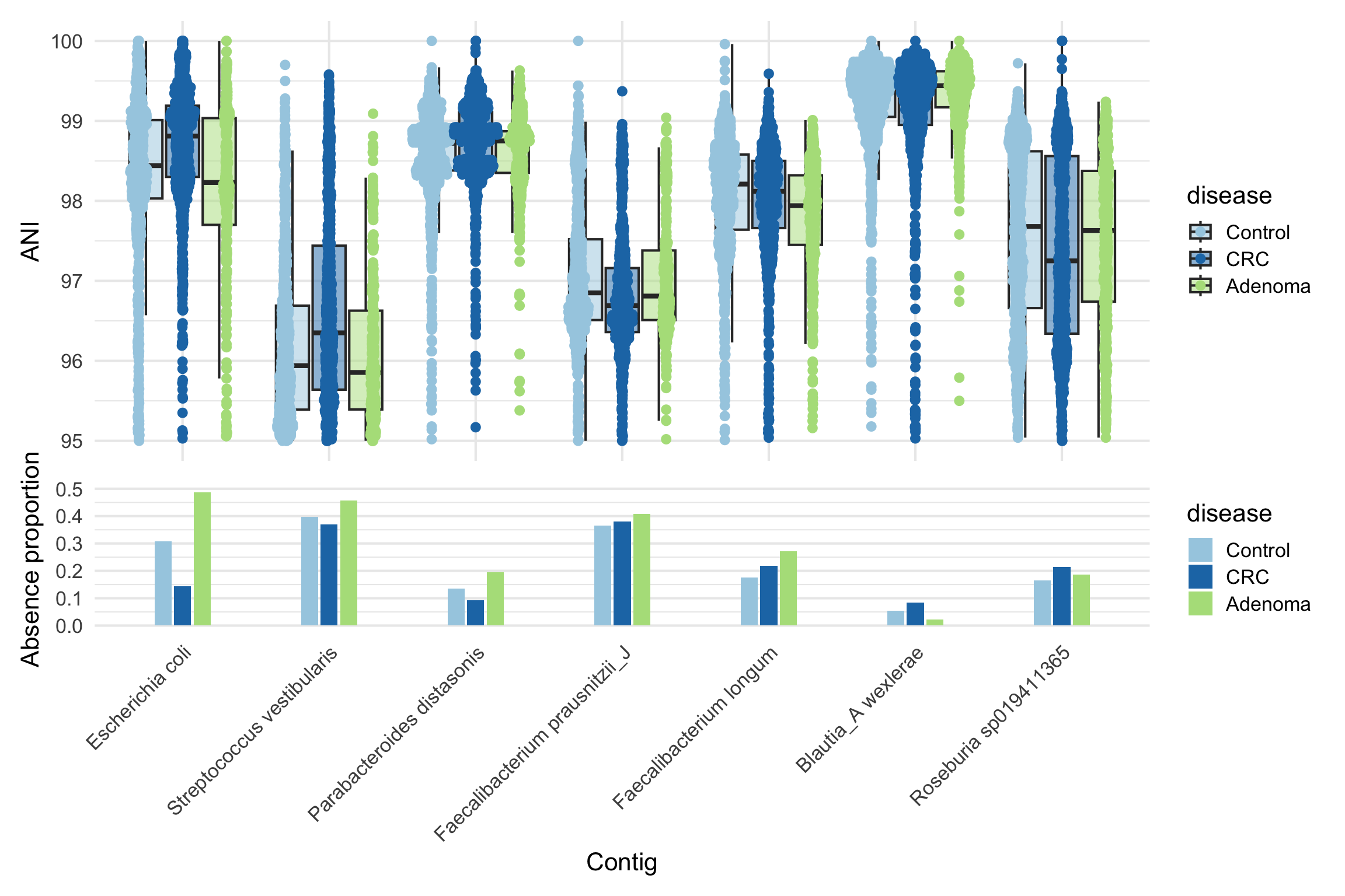
ANI distribution of the top strain of each beta detected species

plot_ani_dist(sy, phenotype = 'disease', contigs = beta_summary$Dominant_contig, 
              show_points = T, plot_type = 'box', 
              contig_names = as.character(beta_summary$Species))

Warning: Removed 5603 rows containing non-finite outside the scale range
(`stat_boxplot()`).

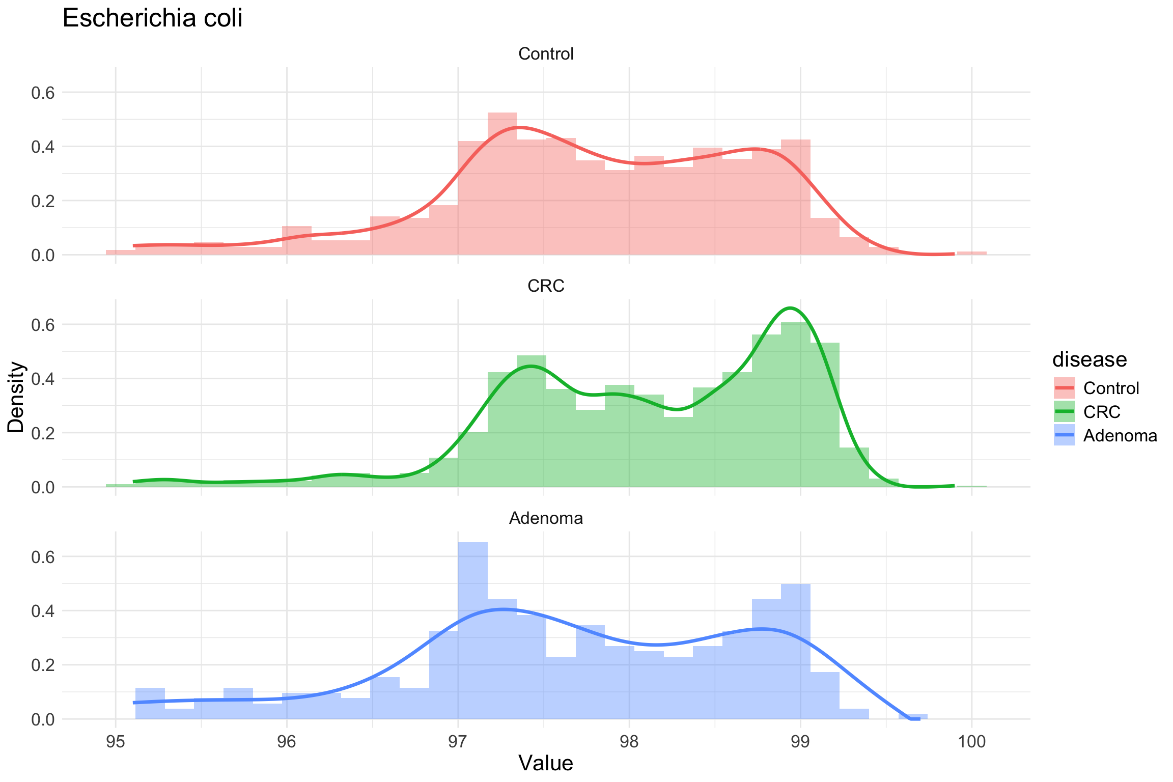
### E coli
th_ec = th[th$Species == "Escherichia coli",]

# Pick a human associated strain
th_ec$Genome_file[11]

[1] "GCF_000458275.1"

# (enasearch) sudarakm@Sudarakas-MacBook-Pro ~ % datasets summary genome accession GCF_000458275.1            
# {"reports": [{"accession":"GCF_000458275.1","annotation_info":{"method":"Best-placed reference protein set; GeneMarkS-2+","name":"GCF_000458275.1-RS_2025_06_14","pipeline":"NCBI Prokaryotic Genome Annotation Pipeline (PGAP)","provider":"NCBI RefSeq","release_date":"2025-06-14","software_version":"6.10","stats":{"gene_counts":{"non_coding":95,"protein_coding":4834,"pseudogene":234,"total":5163}}},"assembly_info":{"assembly_level":"Scaffold","assembly_method":"allpaths v. R46382","assembly_name":"Esch_coli_HVH_153_3-9344314_V1","assembly_status":"current","assembly_type":"haploid","bioproject_accession":"PRJNA186185","bioproject_lineage":[{"bioprojects":[{"accession":"PRJNA186185","parent_accessions":["PRJNA186413"],"title":"E coli UTI Bacteremia"},{"accession":"PRJNA186413","title":"Escherichia coli as human pathogen"}]}],"biosample":{"accession":"SAMN01885798","attributes":[{"name":"geo_loc_name","value":"Denmark"},{"name":"collection_date","value":"2004"},{"name":"host","value":"Homo sapiens"},{"name":"lat_lon","value":"missing"},{"name":"host_disease","value":"UTI induced bacteremia"},{"name":"isolation_source","value":"blood"},{"name":"collected_by","value":"missing"},{"name":"strain","value":"HVH 153 (3-9344314)"}],"bioprojects":[{}],"collected_by":"missing","collection_date":"2004","description":{"organism":{"organism_name":"Escherichia coli HVH 153 (3-9344314)","tax_id":1281086},"title":"Pathogen bacterial, clinical or host-associated sample from Escherichia coli HVH 153 (3-9344314)"},"geo_loc_name":"Denmark","host":"Homo sapiens","host_disease":"UTI induced bacteremia","isolation_source":"blood","last_updated":"2019-05-23T15:25:28.339","lat_lon":"missing","models":["Pathogen.ba-cl"],"owner":{"contacts":[{}],"name":"Broad Institute"},"package":"Pathogen.cl.1.0","publication_date":"2013-01-11T00:00:00.000","sample_ids":[{"label":"Sample name","value":"Escherichia coli HVH 153 (3-9344314)"},{"db":"SRA","value":"SRS399665"}],"status":{"status":"live","when":"2013-01-11T09:27:34.707"},"strain":"HVH 153 (3-9344314)","submission_date":"2013-01-11T09:18:22.980"},"comments":"Please be aware that the annotation is done automatically with little or no manual curation.\nThe annotation was added by the NCBI Prokaryotic Genome Annotation Pipeline (PGAP). Information about PGAP can be found here: https://www.ncbi.nlm.nih.gov/genome/annotation_prok/","paired_assembly":{"accession":"GCA_000458275.1","annotation_name":"Annotation submitted by Broad Institute","status":"current"},"release_date":"2013-08-29","sequencing_tech":"Illumina","submitter":"Broad Institute"},"assembly_stats":{"atgc_count":"5265684","contig_l50":8,"contig_n50":232812,"gc_count":"2656312","gc_percent":50.5,"genome_coverage":"140","number_of_component_sequences":45,"number_of_contigs":45,"number_of_scaffolds":14,"scaffold_l50":3,"scaffold_n50":856756,"total_sequence_length":"5303299","total_ungapped_length":"5265684"},"average_nucleotide_identity":{"best_ani_match":{"ani":98.92,"assembly":"GCA_000013265.1","assembly_coverage":88.06,"category":"claderef","organism_name":"Escherichia coli","type_assembly_coverage":89.52},"category":"category_na","comment":"na","match_status":"species_match","submitted_ani_match":{"ani":98.92,"assembly":"GCA_000013265.1","assembly_coverage":88.06,"category":"claderef","organism_name":"Escherichia coli UTI89","type_assembly_coverage":89.52},"submitted_organism":"Escherichia coli HVH 153 (3-9344314)","submitted_species":"Escherichia coli","taxonomy_check_status":"OK"},"checkm_info":{"checkm_marker_set":"Escherichia coli","checkm_marker_set_rank":"species","checkm_species_tax_id":562,"checkm_version":"v1.2.3","completeness":99,"completeness_percentile":49.7728,"contamination":0.86},"current_accession":"GCF_000458275.1","organism":{"infraspecific_names":{"strain":"HVH 153 (3-9344314)"},"organism_name":"Escherichia coli HVH 153 (3-9344314)","tax_id":1281086},"paired_accession":"GCA_000458275.1","source_database":"SOURCE_DATABASE_REFSEQ","wgs_info":{"master_wgs_url":"https://www.ncbi.nlm.nih.gov/nuccore/AVXM00000000.1","wgs_contigs_url":"https://www.ncbi.nlm.nih.gov/Traces/wgs/AVXM01","wgs_project_accession":"AVXM01"}}],"total_count": 1}


plot_histogram(sy, phenotype = 'disease', contig = th_ec$Contig_name[11],
              drop_zeros = T, show_quantiles = F, fit_spline = T, bins = 30)

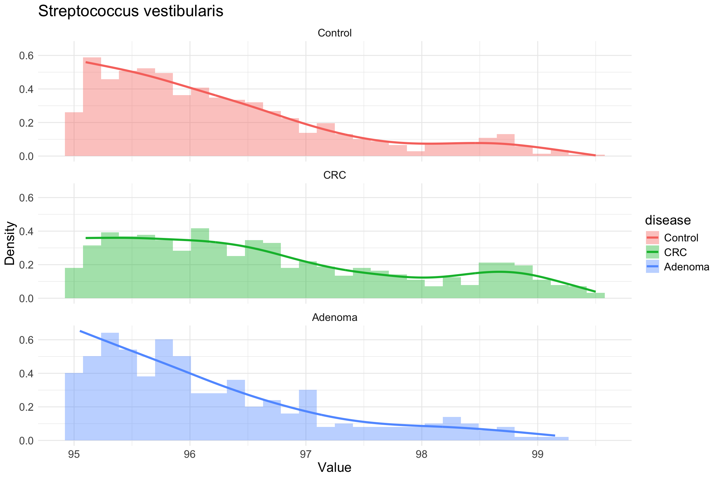
### Streptococcus vestibularis

th_sv = th[th$Species == "Streptococcus vestibularis",]

th_sv$Genome_file[2]

[1] "GCF_958445235.1"

# (enasearch) sudarakm@Sudarakas-MacBook-Pro ~ % datasets summary genome accession GCF_958445235.1                   
# {"reports": [{"accession":"GCF_958445235.1","annotation_info":{"method":"Best-placed reference protein set; GeneMarkS-2+","name":"GCF_958445235.1-RS_2025_07_23","pipeline":"NCBI Prokaryotic Genome Annotation Pipeline (PGAP)","provider":"NCBI RefSeq","release_date":"2025-07-23","software_version":"6.10","stats":{"gene_counts":{"non_coding":38,"protein_coding":1697,"pseudogene":98,"total":1833}}},"assembly_info":{"assembly_level":"Contig","assembly_method":"metaspades v3.15.3","assembly_name":"ERR9609794_bin.7_MetaWRAP_v1.3_MAG","assembly_status":"current","assembly_type":"haploid","bioproject_accession":"PRJEB62825","bioproject_lineage":[{"bioprojects":[{"accession":"PRJEB62825","title":"EMG produced TPA metagenomics assembly of PRJEB21612 data set (Alterations of the gut microbiome in hypertension)."}]}],"biosample":{"accession":"SAMEA114061883","attributes":[{"name":"ENA-CHECKLIST","value":"ERC000047"},{"name":"ENA-FIRST-PUBLIC","value":"2023-07-13T16:22:57Z"},{"name":"ENA-LAST-UPDATE","value":"2023-07-13T16:22:57Z"},{"name":"External Id","value":"SAMEA114061883"},{"name":"INSDC center alias","value":"EMG"},{"name":"INSDC center name","value":"EMG"},{"name":"INSDC first public","value":"2023-07-13T16:22:57Z"},{"name":"INSDC last update","value":"2023-07-13T16:22:57Z"},{"name":"INSDC status","value":"public"},{"name":"Submitter Id","value":"ERR9609794_bin.7_MetaWRAP_v1.3_MAG"},{"name":"assembly quality","value":"Many fragments with little to no review of assembly other than reporting of standard assembly statistics"},{"name":"assembly software","value":"metaspades v3.15.3"},{"name":"binning parameters","value":"MaxBin2, MetaBat2, Concoct with default parameter of the metaWRAP pipeline. Bin refinement module used from metaWRAP with default parameters."},{"name":"binning software","value":"MetaWRAP v1.3"},{"name":"env_broad_scale","value":"Human digestive system"},{"name":"broker name","value":"EMG broker account, EMBL-EBI"},{"name":"collection_date","value":"2015"},{"name":"completeness score","value":"97.8"},{"name":"completeness software","value":"CheckM"},{"name":"contamination score","value":"1.42"},{"name":"env_medium","value":"faeces"},{"name":"geo_loc_name","value":"China"},{"name":"geographic location (latitude)","value":"39.0"},{"name":"geographic location (longitude)","value":"122.0"},{"name":"investigation_type","value":"metagenome-assembled genome"},{"name":"isolation_source","value":"human feces metagenome"},{"name":"local environmental context","value":"colon"},{"name":"metagenomic source","value":"human feces metagenome"},{"name":"project_name","value":"Human gut microbiota is believed to be directly or indirectly involved in cardiovascular diseases and hypertension. However, the identification and functional status of the hypertension-related gut microbe(s) have not yet been surveyed in a comprehensive manner. Here we characterized the gut microbiome in hypertension status by comparing fecal samples of 60 patients with primary hypertension and 60 gender-, age-, and body weight-matched healthy controls based on whole-metagenome shotgun sequencing."},{"name":"sample derived from","value":"SAMEA14093502"},{"name":"sample_name","value":"ERR9609794_bin.7_MetaWRAP_v1.3_MAG"},{"name":"scientific_name","value":"Streptococcus vestibularis"},{"name":"sequencing method","value":"Illumina HiSeq 2000"},{"name":"taxonomic classification","value":"The taxonomy of this Metagenome-Assembled Genome was originally computed with GTDBtk, which assigned the following taxonomic annotation: d__Bacteria;p__Firmicutes;c__Bacilli;o__Lactobacillales;f__Streptococcaceae;g__Streptococcus;s__Streptococcus vestibularis"},{"name":"taxonomic identity marker","value":"multi-marker approach"}],"collection_date":"2015","description":{"comment":"This sample represents a Third Party Annotation (TPA) metagenome-assembled genome assembled from the metagenomic run ERR9609794 of study ERP023883.","organism":{"organism_name":"Streptococcus vestibularis","tax_id":1343},"title":"Metagenome-Assembled Genome: ERR9609794_bin.7_MetaWRAP_v1.3_MAG"},"geo_loc_name":"China","isolation_source":"human feces metagenome","last_updated":"2023-07-15T06:13:51.000","models":["Generic"],"owner":{"name":"EBI"},"package":"Generic.1.0","project_name":"Human gut microbiota is believed to be directly or indirectly involved in cardiovascular diseases and hypertension. However, the identification and functional status of the hypertension-related gut microbe(s) have not yet been surveyed in a comprehensive manner. Here we characterized the gut microbiome in hypertension status by comparing fecal samples of 60 patients with primary hypertension and 60 gender-, age-, and body weight-matched healthy controls based on whole-metagenome shotgun sequencing.","publication_date":"2023-07-13T00:00:00.000","sample_ids":[{"db":"SRA","value":"ERS16045747"}],"sample_name":"ERR9609794_bin.7_MetaWRAP_v1.3_MAG","status":{"status":"live","when":"2023-07-17T10:07:32.262"},"submission_date":"2023-07-17T10:07:32.262"},"comments":"The annotation was added by the NCBI Prokaryotic Genome Annotation Pipeline (PGAP). Information about PGAP can be found here: https://www.ncbi.nlm.nih.gov/genome/annotation_prok/","genome_notes":["derived from metagenome"],"paired_assembly":{"accession":"GCA_958445235.1","status":"current"},"release_date":"2023-07-18","sequencing_tech":"Illumina HiSeq 2000","submitter":"EMG"},"assembly_stats":{"atgc_count":"1832103","contig_l50":14,"contig_n50":42507,"gc_count":"725658","gc_percent":39.5,"genome_coverage":"101","number_of_component_sequences":72,"number_of_contigs":72,"number_of_scaffolds":72,"scaffold_l50":14,"scaffold_n50":42507,"total_sequence_length":"1832103","total_ungapped_length":"1832103"},"average_nucleotide_identity":{"best_ani_match":{"ani":97.14,"assembly":"GCA_053203075.1","assembly_coverage":89.61,"category":"type","organism_name":"Streptococcus vestibularis","type_assembly_coverage":87.66},"category":"category_na","comment":"na","match_status":"species_match","submitted_ani_match":{"ani":97.14,"assembly":"GCA_053203075.1","assembly_coverage":89.61,"category":"type","organism_name":"Streptococcus vestibularis","type_assembly_coverage":87.66},"submitted_organism":"Streptococcus vestibularis","submitted_species":"Streptococcus vestibularis","taxonomy_check_status":"OK"},"checkm_info":{"checkm_marker_set":"Streptococcus","checkm_marker_set_rank":"genus","checkm_species_tax_id":1343,"checkm_version":"v1.2.4","completeness":96.77,"completeness_percentile":20.7547,"contamination":0.4},"current_accession":"GCF_958445235.1","organism":{"infraspecific_names":{"isolate":"ERR9609794_bin.7_MetaWRAP_v1.3_MAG"},"organism_name":"Streptococcus vestibularis","tax_id":1343},"paired_accession":"GCA_958445235.1","source_database":"SOURCE_DATABASE_REFSEQ","wgs_info":{"master_wgs_url":"https://www.ncbi.nlm.nih.gov/nuccore/CAUCRO000000000.1","wgs_contigs_url":"https://www.ncbi.nlm.nih.gov/Traces/wgs/CAUCRO01","wgs_project_accession":"CAUCRO01"}}],"total_count": 1}

plot_histogram(sy, phenotype = 'disease', contig = th_sv$Contig_name[2],
              drop_zeros = T, show_quantiles = F, fit_spline = T, bins = 30)

Associations with other metadata

Since tumour_stage_AJCC and tumour_location are highly correlated with disease, we’ll first fit separate models on subsets for direct comparison.

Tumour location

# Directly compare left vs. right
meta_lr_acc = which(meta$tumour_location == 'left_sided' | meta$tumour_location == 'right_sided')
lr_acc = meta$run_accession[meta_lr_acc]
meta_lr = meta[meta_lr_acc, c('run_accession', 'study', 'age', 'BMI', 'sex', 'tumour_location')]
meta_lr$tumour_location = factor(as.character(meta_lr$tumour_location), levels = c('left_sided', 'right_sided'))
# Reload sylph q99
sy <- read_sylph("./data/segata_pooled_3741/combined_q_99.tsv.gz") # q99)

Detected Sylph query output file.

# annoying renames to match meta V sylph file
colnames(sy) <- gsub("_1", "", colnames(sy))
colnames(sy) <- gsub("_merged", "", colnames(sy))
colData(sy)$Sample_file <- gsub("_1", "", basename(colData(sy)$Sample_file))
colData(sy)$Sample_file <- gsub("_merged", "", colnames(sy))

# only lVr samples
sy = sy[, sapply(lr_acc, function(x) which(x == colnames(sy)))]
sy <- filter_by_presence(sy, min_nonzero = round(dim(sy)[2]/10)) # filter at 10%

Retained 21496 rows after filtering

dim(sy)

[1] 21496   868

# Checks before merging metadata
all(colnames(sy) %in% meta_lr$run_accession)

[1] TRUE

all(meta_lr$run_accession %in% colnames(sy))

[1] TRUE

sy = modify_metadata(sy, meta_lr)

design <- as.formula("~ tumour_location + age + sex + BMI + (1 | study)")

save_path <- "output_rds/CRC_zib_q_99_ebp_tumour_location_lVr.rds"
# Run with ebp - this looks a bit less noisy
if(file.exists(save_path)){
  ZB_fit_tl <- readRDS(save_path)
} else {
  ebp = compute_eb_priors(sy, strainspy:::nobars_(design), nthreads = parallel::detectCores(),low_cutoff = 0, high_cutoff = Inf)
  ZB_fit_tl <- glmZiBFit(sy,  design, MAP_prior = ebp, nthreads = parallel::detectCores())
  saveRDS(ZB_fit_tl, save_path)
}

Build a summary from top hits

th_tl = top_hits(ZB_fit_tl, coef = 2)

Found 81 tophits for tumour_locationright_sided at alpha = 0.05 using holm 

# There are no strain identity differences, post hoc testing ignored

th_tl$Species = taxonomy$Species[match(th_tl$Genome_file, taxonomy$Genome)]

# Signals detected from 11 species
length(sort(table(th_tl$Species), decreasing = T))

[1] 11

# Ask chatGPT for a nice summary table
summary_tbl <- th_tl %>%
  filter(!is.na(Species)) %>%
  group_by(Species) %>%
  summarise(
    N_hits = n(),
    
    Top_adj_p_beta  = min(p_adjust, na.rm = TRUE),
    Top_coef_beta   = coefficient[which.min(p_adjust)],
    Top_se_beta     = std_error[which.min(p_adjust)],
    Top_contig_beta = Contig_name[which.min(p_adjust)],
    
    Top_adj_p_ZI    = min(zi_p_adjust, na.rm = TRUE),
    Top_coef_ZI     = zi_coefficient[which.min(zi_p_adjust)],
    Top_se_ZI       = zi_std_error[which.min(zi_p_adjust)],
    Top_contig_ZI   = Contig_name[which.min(zi_p_adjust)],
    
    .groups = "drop"
  ) %>%
  mutate(
    Min_adj_p = pmin(Top_adj_p_beta, Top_adj_p_ZI, na.rm = TRUE),
    Dominant_component = ifelse(Top_adj_p_beta < Top_adj_p_ZI, "Beta", "ZI"),
    Dominant_contig    = ifelse(Dominant_component == "Beta", Top_contig_beta, Top_contig_ZI),
    Dominant_coef      = ifelse(Dominant_component == "Beta", Top_coef_beta, Top_coef_ZI),
    Dominant_se        = ifelse(Dominant_component == "Beta", Top_se_beta, Top_se_ZI)
  ) %>%
  select(Species, N_hits, Dominant_component, Min_adj_p, Dominant_coef, Dominant_se, Dominant_contig) %>%
  arrange(Min_adj_p)

# Write as tsv for manual perusal
# write.table(summary_tbl, "output_tables/CRC_Z99_tVl_direct_summary.tsv", sep = '\t', col.names = T, row.names = F, quote = F)

There are only presence/absence hits.

ZI component hits

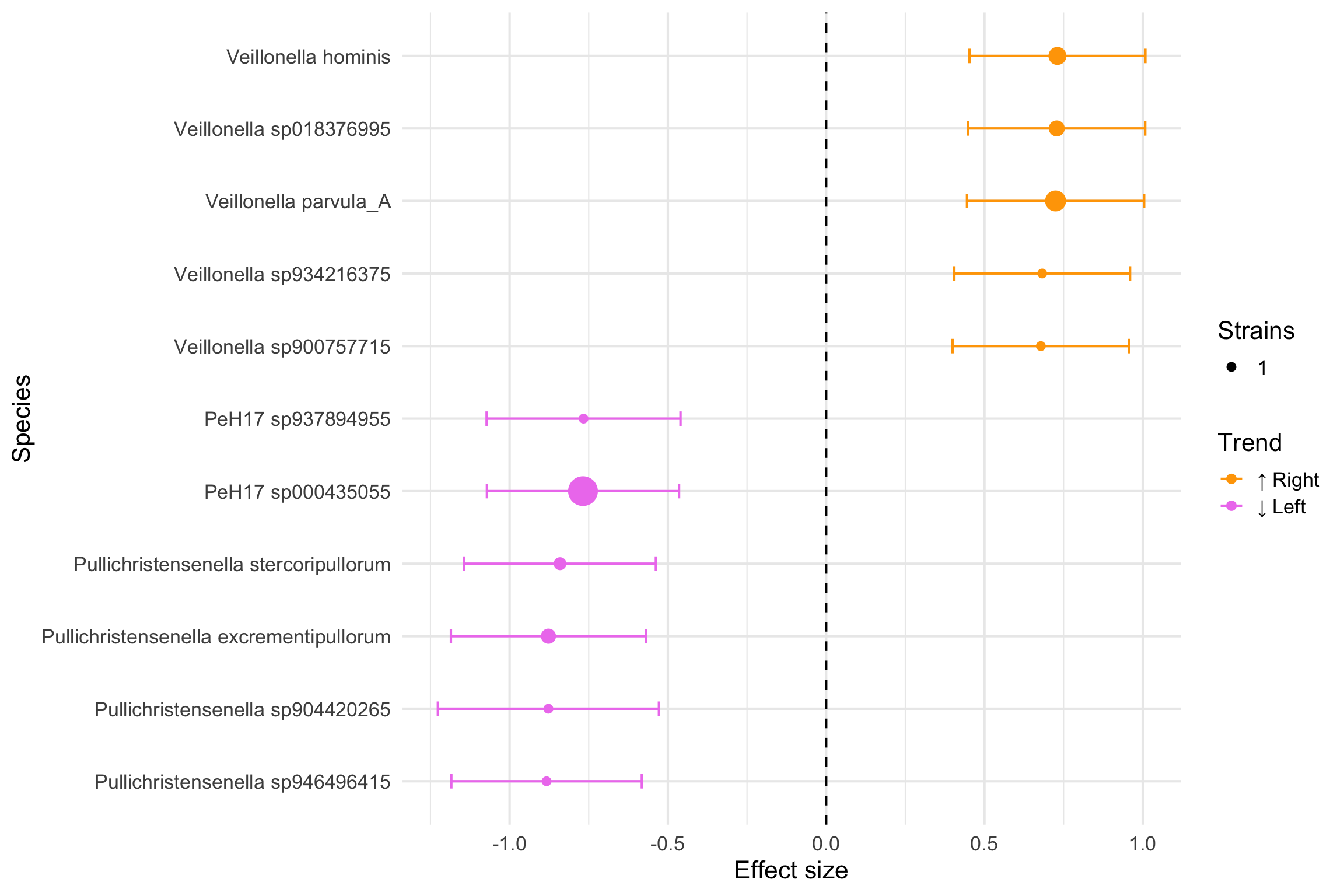
Negative and positive Dominant_coef indicates strain presence in the guts of patients with Left and Right CRC tumors, respectively.

Visualise this in a forest plot

zi_summary <- summary_tbl %>%
  filter(Dominant_component == "ZI") %>%
  arrange(Min_adj_p) %>%
  mutate(
    # Confidence interval before flipping
    CI_low = Dominant_coef - 1.96 * Dominant_se,
    CI_high = Dominant_coef + 1.96 * Dominant_se,
    
    # Flip effect size and CI
    Dominant_coef = -Dominant_coef,
    CI_low = -CI_low,
    CI_high = -CI_high,
    
    # Trend annotation
    Trend = ifelse(Dominant_coef > 0, "\u2191 Right", "\u2193 Left")
  ) %>%
  arrange(Trend, desc(Dominant_coef)) %>%
  mutate(Species = factor(Species, levels = rev(unique(Species))))

ggplot(zi_summary, aes(x = Dominant_coef, y = Species, color = Trend)) +
  geom_point(aes(size = N_hits)) +
  geom_errorbarh(aes(xmin = CI_low, xmax = CI_high), height = 0.2) +
  geom_vline(xintercept = 0, linetype = "dashed") +
  scale_color_manual(values = c("\u2191 Right" = "orange", "\u2193 Left" = "violet")) +
  scale_size_continuous(
    name = "Strains",
    range = c(2, 8),  # tweak for your figure aesthetics
    breaks = c(1, 45, 90),
    labels = c("1", "45", "90"),
    guide = guide_legend(override.aes = list(linetype = 0))  # remove lines from legend
  ) +
  labs(
    x = "Effect size",
    y = "Species",
    color = "Trend"
  ) +
  theme_minimal(base_size = 16)

`height` was translated to `width`.

Looks like it is mostly dominated by Veillonella sp. and Pullichristensenella sp.. Veillonella parvula is one of the top hits in 10.1016/j.chom.2025.03.012, but we are not detecting any of the other hits.

Cancer stage

table(meta$tumour_stage_AJCC)

NoTumour  Adenoma        0        I       II      III       IV Unstaged 
    1478      614       90      231      230      258      289      224 

# Directly compare left vs. right
meta_stage_acc = which(meta$tumour_stage_AJCC == '0' | 
                         meta$tumour_stage_AJCC == 'I' | 
                         meta$tumour_stage_AJCC == 'II' | 
                         meta$tumour_stage_AJCC == 'III' | 
                         meta$tumour_stage_AJCC == 'IV')

stage_acc = meta$run_accession[meta_stage_acc]
meta_stage = meta[meta_stage_acc, c('run_accession', 'study', 'age', 'BMI', 'sex', 'tumour_stage_AJCC')]
meta_stage$tumour_stage_AJCC = factor(as.character(meta_stage$tumour_stage_AJCC), levels = c('0', 'I', 'II', 'III', 'IV'))

###################
##### No HITS #####
###################
#### Model 1 - compare stages 1,2,3 and 4 vs. stage 0
# Reload sylph q99
sy <- read_sylph("./data/segata_pooled_3741/combined_q_99.tsv.gz") # q99)

Detected Sylph query output file.

# annoying renames to match meta V sylph file
colnames(sy) <- gsub("_1", "", colnames(sy))
colnames(sy) <- gsub("_merged", "", colnames(sy))
colData(sy)$Sample_file <- gsub("_1", "", basename(colData(sy)$Sample_file))
colData(sy)$Sample_file <- gsub("_merged", "", colnames(sy))

# only lVr samples
sy = sy[, sapply(meta_stage$run_accession, function(x) which(x == colnames(sy)))]
sy <- filter_by_presence(sy, min_nonzero = round(dim(sy)[2]/10)) # filter at 10%

Retained 21722 rows after filtering

dim(sy)

[1] 21722  1098

# Checks before merging metadata
all(colnames(sy) %in% meta_stage$run_accession)

[1] TRUE

all(meta_stage$run_accession %in% colnames(sy))

[1] TRUE

sy = modify_metadata(sy, meta_stage)


save_path <- "output_rds/CRC_zib_q_99_ebp_tumour_stage_0v.rds"
design <- as.formula('~tumour_stage_AJCC + age + sex + BMI + (1 | study)')
# Run with ebp
if(file.exists(save_path)){
  ZB_fit_stage_full <- readRDS(save_path)
} else {
  ebp = compute_eb_priors(sy, strainspy:::nobars_(design), nthreads = parallel::detectCores(),low_cutoff = 0, high_cutoff = Inf)
  ZB_fit_stage_full <- glmZiBFit(sy,  design, MAP_prior = ebp, nthreads = parallel::detectCores())
  saveRDS(ZB_fit_stage_full, save_path)
}

# Variables
top_hits(ZB_fit_stage_full, coef = 2, method = "BH")

Warning in top_hits(ZB_fit_stage_full, coef = 2, method = "BH"): Multiple
testing correction using `BH`: No significant associations detected for coef =
2 at alpha = 0.050000

# A tibble: 0 × 10
# ℹ 10 variables: Contig_name <chr>, Genome_file <chr>, coefficient <dbl>,
#   std_error <dbl>, p_value <dbl>, p_adjust <dbl>, zi_coefficient <dbl>,
#   zi_std_error <dbl>, zi_p_value <dbl>, zi_p_adjust <dbl>

top_hits(ZB_fit_stage_full, coef = 3, method = "BH")

Warning in top_hits(ZB_fit_stage_full, coef = 3, method = "BH"): Multiple
testing correction using `BH`: No significant associations detected for coef =
3 at alpha = 0.050000

# A tibble: 0 × 10
# ℹ 10 variables: Contig_name <chr>, Genome_file <chr>, coefficient <dbl>,
#   std_error <dbl>, p_value <dbl>, p_adjust <dbl>, zi_coefficient <dbl>,
#   zi_std_error <dbl>, zi_p_value <dbl>, zi_p_adjust <dbl>

top_hits(ZB_fit_stage_full, coef = 4, method = "BH")

Warning in top_hits(ZB_fit_stage_full, coef = 4, method = "BH"): Multiple
testing correction using `BH`: No significant associations detected for coef =
4 at alpha = 0.050000

# A tibble: 0 × 10
# ℹ 10 variables: Contig_name <chr>, Genome_file <chr>, coefficient <dbl>,
#   std_error <dbl>, p_value <dbl>, p_adjust <dbl>, zi_coefficient <dbl>,
#   zi_std_error <dbl>, zi_p_value <dbl>, zi_p_adjust <dbl>

top_hits(ZB_fit_stage_full, coef = 5, method = "BH")

Warning in top_hits(ZB_fit_stage_full, coef = 5, method = "BH"): Multiple
testing correction using `BH`: No significant associations detected for coef =
5 at alpha = 0.050000

# A tibble: 0 × 10
# ℹ 10 variables: Contig_name <chr>, Genome_file <chr>, coefficient <dbl>,
#   std_error <dbl>, p_value <dbl>, p_adjust <dbl>, zi_coefficient <dbl>,
#   zi_std_error <dbl>, zi_p_value <dbl>, zi_p_adjust <dbl>

#### Model 2 - merge stages 0 and 1 as early and compare with 2, 3 and 4.
###################
##### HAS HITS ####
###################
meta_stage$tumour_stage_merged = sapply(as.character(meta_stage$tumour_stage_AJCC), function(x) ifelse( (x=='0'|x=='I'), 'Early', x)) 
meta_stage$tumour_stage_merged = factor(as.character(meta_stage$tumour_stage_merged), levels = c('Early', 'II', 'III', 'IV'))

save_path <- "output_rds/CRC_zib_q_99_ebp_tumour_stage_early0Iv.rds"
design <- as.formula('~tumour_stage_merged + age + sex + BMI + (1 | study)')
sy = modify_metadata(sy, meta_stage)

Warning in modify_metadata(sy, meta_stage): The following metadata columns already exist in `se` and will not be modified. To replace with provided meta_data, set run again with `replace = TRUE`:

study, age, BMI, sex, tumour_stage_AJCC

# Run with ebp
if(file.exists(save_path)){
  ZB_fit_stage_early012V <- readRDS(save_path)
} else {
  ebp = compute_eb_priors(sy, strainspy:::nobars_(design), nthreads = parallel::detectCores(),low_cutoff = 0, high_cutoff = Inf)
  ZB_fit_stage_early012V <- glmZiBFit(sy,  design, MAP_prior = ebp, nthreads = parallel::detectCores())
  saveRDS(ZB_fit_stage_early012V, save_path)
}

# Variables
th_stage_1 = cbind(top_hits(ZB_fit_stage_early012V, coef = 2, method = "BH"), model = 'early01V', stage = 2)

Found 24 tophits for tumour_stage_mergedII at alpha = 0.05 using BH 

top_hits(ZB_fit_stage_early012V, coef = 3, method = "BH")

Warning in top_hits(ZB_fit_stage_early012V, coef = 3, method = "BH"): Multiple
testing correction using `BH`: No significant associations detected for coef =
3 at alpha = 0.050000

# A tibble: 0 × 10
# ℹ 10 variables: Contig_name <chr>, Genome_file <chr>, coefficient <dbl>,
#   std_error <dbl>, p_value <dbl>, p_adjust <dbl>, zi_coefficient <dbl>,
#   zi_std_error <dbl>, zi_p_value <dbl>, zi_p_adjust <dbl>

th_stage_2 = cbind(top_hits(ZB_fit_stage_early012V, coef = 4, method = "BH"), model = 'early01V', stage = 4)

Found 14 tophits for tumour_stage_mergedIV at alpha = 0.05 using BH 

#### No results - Fig 3B from Segata paper - merge 0, 1 and 2 as early and compare with merged 3 and 4 (late)
meta_stage$tumour_stage_merged_earlyVlate = sapply(as.character(meta_stage$tumour_stage_AJCC), function(x) ifelse( (x=='0'|x=='I'|x=='II'), 'Early', 'Late')) 
meta_stage$tumour_stage_merged_earlyVlate = factor(as.character(meta_stage$tumour_stage_merged_earlyVlate), levels = c('Early', 'Late'))

save_path <- "output_rds/CRC_zib_q_99_ebp_tumour_stage_early012Vlate34.rds"
design <- as.formula('~tumour_stage_merged_earlyVlate + age + sex + BMI + (1 | study)')
sy = modify_metadata(sy, meta_stage)

Warning in modify_metadata(sy, meta_stage): The following metadata columns already exist in `se` and will not be modified. To replace with provided meta_data, set run again with `replace = TRUE`:

study, age, BMI, sex, tumour_stage_AJCC, tumour_stage_merged

# Run with ebp
if(file.exists(save_path)){
  ZB_fit_stage_early012Vlate34 <- readRDS(save_path)
} else {
  ebp = compute_eb_priors(sy, strainspy:::nobars_(design), nthreads = parallel::detectCores(),low_cutoff = 0, high_cutoff = Inf)
  ZB_fit_stage_early012Vlate34 <- glmZiBFit(sy,  design, MAP_prior = ebp, nthreads = parallel::detectCores())
  saveRDS(ZB_fit_stage_early012Vlate34, save_path)
}

# Variables
top_hits(ZB_fit_stage_early012Vlate34, coef = 2, method = "BH")

Warning in top_hits(ZB_fit_stage_early012Vlate34, coef = 2, method = "BH"):
Multiple testing correction using `BH`: No significant associations detected
for coef = 2 at alpha = 0.050000

# A tibble: 0 × 10
# ℹ 10 variables: Contig_name <chr>, Genome_file <chr>, coefficient <dbl>,
#   std_error <dbl>, p_value <dbl>, p_adjust <dbl>, zi_coefficient <dbl>,
#   zi_std_error <dbl>, zi_p_value <dbl>, zi_p_adjust <dbl>

#### Has results - Fig 3C from Segata paper - merge 0, 1, 2, 3 as early and compare with 4
meta_stage$tumour_stage_merged_early3Vlate = sapply(as.character(meta_stage$tumour_stage_AJCC), function(x) ifelse( (x=='0'|x=='I'|x=='II'|x=="III"), 'Early', x)) 
meta_stage$tumour_stage_merged_early3Vlate = factor(as.character(meta_stage$tumour_stage_merged_early3Vlate), levels = c('Early', 'IV'))
sy = modify_metadata(sy, meta_stage)

Warning in modify_metadata(sy, meta_stage): The following metadata columns already exist in `se` and will not be modified. To replace with provided meta_data, set run again with `replace = TRUE`:

study, age, BMI, sex, tumour_stage_AJCC, tumour_stage_merged, tumour_stage_merged_earlyVlate

save_path <- "output_rds/CRC_zib_q_99_ebp_tumour_stage_early0123V4.rds"
design <- as.formula('~tumour_stage_merged_early3Vlate + age + sex + BMI + (1 | study)')

# Run with ebp
if(file.exists(save_path)){
  ZB_fit_stage_early0123V4 <- readRDS(save_path)
} else {
  ebp = compute_eb_priors(sy, strainspy:::nobars_(design), nthreads = parallel::detectCores(),low_cutoff = 0, high_cutoff = Inf)
  ZB_fit_stage_early0123V4 <- glmZiBFit(sy,  design, MAP_prior = ebp, nthreads = parallel::detectCores())
  saveRDS(ZB_fit_stage_early0123V4, save_path)
}


# Variables
th_stage_3 = cbind(top_hits(ZB_fit_stage_early0123V4, coef = 2, method = "BH"), model = 'early0123V', stage = 4)

Found 5 tophits for tumour_stage_merged_early3VlateIV at alpha = 0.05 using BH 

th_stage = rbind(th_stage_1, th_stage_2, th_stage_3)
th_stage$Species = taxonomy$Species[match(th_stage$Genome_file, taxonomy$Genome)]


summary_tbl <- th_stage %>%
  filter(!is.na(Species)) %>%
  group_by(Species, stage) %>%
  summarise(
    N_hits = n(), 
    
    Top_adj_p_beta  = min(p_adjust, na.rm = TRUE),
    Top_coef_beta   = coefficient[which.min(p_adjust)],
    Top_se_beta     = std_error[which.min(p_adjust)],
    Top_contig_beta = Contig_name[which.min(p_adjust)],
    
    Top_adj_p_ZI    = min(zi_p_adjust, na.rm = TRUE),
    Top_coef_ZI     = zi_coefficient[which.min(zi_p_adjust)],
    Top_se_ZI       = zi_std_error[which.min(zi_p_adjust)],
    Top_contig_ZI   = Contig_name[which.min(zi_p_adjust)],
    
    .groups = "drop"
  ) %>%
  mutate(
    stage = stage,
    Min_adj_p = pmin(Top_adj_p_beta, Top_adj_p_ZI, na.rm = TRUE),
    Dominant_component = ifelse(Top_adj_p_beta < Top_adj_p_ZI, "Beta", "ZI"),
    Dominant_contig    = ifelse(Dominant_component == "Beta", Top_contig_beta, Top_contig_ZI),
    Dominant_coef      = ifelse(Dominant_component == "Beta", Top_coef_beta, Top_coef_ZI),
    Dominant_se        = ifelse(Dominant_component == "Beta", Top_se_beta, Top_se_ZI)
  ) %>%
  select(Species, N_hits, stage, Dominant_component, Min_adj_p, Dominant_coef, Dominant_se, Dominant_contig) %>%
  arrange(Min_adj_p)

# Write as tsv for manual perusal
# write.table(summary_tbl, "output_tables/CRC_Z99_ebp_stage_hits_summary.tsv", sep = '\t', col.names = T, row.names = F, quote = F)

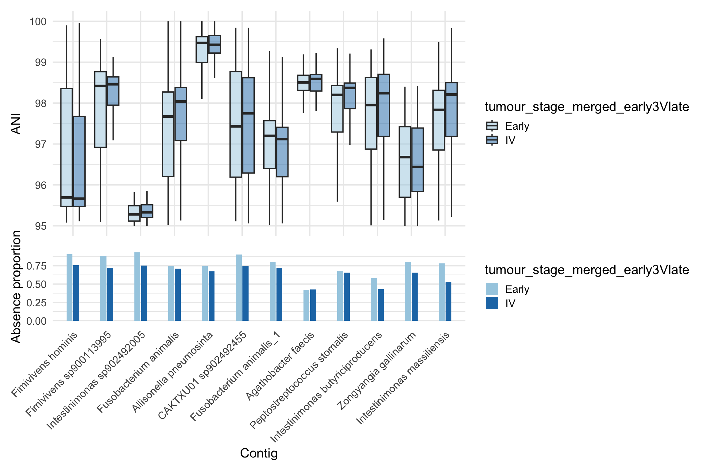
plot_ani_dist(sy, phenotype = 'tumour_stage_merged_early3Vlate', contigs = summary_tbl$Dominant_contig, plot_type = 'box', show_points = F, contig_names = strainspy:::clean_contig_names(summary_tbl$Species))

Warning: Removed 9680 rows containing non-finite outside the scale range
(`stat_boxplot()`).

Warning: No shared levels found between `names(values)` of the manual scale and the
data's colour values.

In short, it looks like species such as Fusobacterium animalis, Peptostreptococcus stomatis and Allisonella pneumosintes grow in prevalence as CRC progresses from very early stages and remains stable. Beneficial species such as Agathobacter faecis seems to get replaced by other different strains at later stages - possibly consistent with treatment intensity.

Paper figures

#  Some files are missing to generate these, but these are optional
# # For CRC ZI signals, let's show the presence absence (<95% ANI) as a tile plot
# zi_summary$Dominant_contig[order(abs(zi_summary$Dominant_coef), decreasing = T)[1:5]]
# 
# # Which ones to use:
# # Dialister pneumosintes - NZ_CP017037.1
# # Peptostreptococcus stomatis - NZ_ADGQ01000074.1
# # Gemella morbillorum - NZ_LS483440.1
# # Parvimonas micra - NZ_LR134472.1
# # Fusobacterium animalis - NZ_CP071098.1
# 
# # Roseburia rectibacter - NZ_CP092473.1
# 
# zib_contigs = c("NZ_CP017037.1", "NZ_ADGQ01000074.1", "NZ_LS483440.1", "NZ_LR134472.1", "NZ_CP071098.1", 
#                 "CAKRCB010000001.1", "CABUSM010000001.1", "CAKRGY010000001.1", "CAUDRE010000001.1", "NZ_QUJS01000001.1")
# sy_ss = sy[sapply(zib_contigs, function(x) grep(x, rownames(sy))),]
# 
# prev_ = list()
# for(i in c("CRC", "Control")){
#   sy_ss_t = as.matrix(assay(subset(sy_ss, select = colData(sy_ss)$disease  %in% i)))
#   prev_[[i]] = apply(sy_ss_t, 1, function(x) sum(x >= 95)/ncol(sy_ss_t))
# }
# prev_df = data.frame(do.call(cbind, prev_))
# prev_df$Species = c("Dialister pneumosintes", 
#                     "Peptostreptococcus stomatis",
#                     "Gemella morbillorum",
#                     "Parvimonas micra",
#                     "Fusobacterium animalis",
#                     "Lachnospira sp.",
#                     "Faecalibacterium sp.",
#                     "Butyribacter hominis",
#                     "Faecalibacterium prausnitzii",
#                     "Butyribacter intestini")
# 
# 
# prev_df <- prev_df %>%
#   mutate(
#     log2FC = log2(CRC / Control),
#     direction = ifelse(log2FC > 0, "Enriched in CRC", "Depleted in CRC")
#   )
# 
# # explicit ordering: CRC group first (high to low), then Control group
# crc_df <- prev_df %>%
#   filter(direction == "Enriched in CRC") %>%
#   arrange(desc(CRC))
# 
# ctrl_df <- prev_df %>%
#   filter(direction == "Depleted in CRC") %>%
#   arrange(CRC)
# 
# prev_df$Species <- factor(
#   prev_df$Species,
#   levels = c(ctrl_df$Species, crc_df$Species)
# )
# 
# ggplot(prev_df, aes(y = Species)) +
#   
#   geom_segment(
#     aes(x = Control, xend = CRC, yend = Species, color = direction),
#     linewidth = 1.2
#   ) +
#   
#   geom_point(aes(x = Control, color = direction),
#              shape = 21, fill = "white", size = 3) +
#   
#   geom_point(aes(x = CRC, color = direction),
#              shape = 21, fill = "black", size = 3) +
#   
#   scale_color_manual(values = c(
#     "Enriched in CRC" = "#d73027",
#     "Depleted in CRC" = "#4575b4"
#   )) +
#   
#   labs(x = "Prevalence", y = NULL, color = NULL) +
#   
#   theme_classic(base_size = 16) +   # 👈 main change
#   
#   theme(
#     axis.text.y = element_text(size = 14),
#     axis.text.x = element_text(size = 13),
#     axis.title.x = element_text(size = 15, face = "bold"),
#     
#     legend.position = "top",
#     legend.text = element_text(size = 13),
#     
#     axis.line = element_line(linewidth = 0.7)
#   )
# 
# #####################################
# do_lolipop = function(th_sp){
#   
#   library(dplyr)
#   library(tidyr)
#   library(ggplot2)
#   
#   ## =========================================================
#   ## species name
#   ## =========================================================
#   
#   species_name = unique(th_sp$Species)
#   
#   ## =========================================================
#   ## get submatrices
#   ## =========================================================
#   
#   sy_ec = sy[
#     sapply(
#       th_sp$Contig_name,
#       function(x) which(rownames(sy) %in% x)
#     ),
#   ]
#   
#   sy_ec_crc = as.matrix(
#     assay(
#       subset(
#         sy_ec,
#         select = colData(sy_ec)$disease %in% "CRC"
#       )
#     )
#   )
#   
#   sy_ec_ctr = as.matrix(
#     assay(
#       subset(
#         sy_ec,
#         select = colData(sy_ec)$disease %in% "Control"
#       )
#     )
#   )
#   
#   ## =========================================================
#   ## mean ANI per strain
#   ## =========================================================
#   
#   crc_mean <- apply(
#     sy_ec_crc,
#     1,
#     function(x)
#       mean(x[x > 0], na.rm = TRUE)
#   )
#   
#   ## reconstruct HC from model-estimated contrast
#   hc_mean <- crc_mean - th_sp$ANI_Difference
#   
#   ## =========================================================
#   ## plotting dataframe
#   ## =========================================================
#   
#   df_plot <- data.frame(
#     strain = names(hc_mean),
#     HC = hc_mean,
#     CRC = crc_mean,
#     effect = th_sp$ANI_Difference,
#     padj = th_sp$p_adjust
#   )
#   
#   ## direction
#   df_plot$direction <- df_plot$CRC > df_plot$HC
#   
#   ## WLS weights
#   df_plot$weights <- -log10(df_plot$padj + 1e-10)
#   
#   ## avoid zero / inf weirdness
#   df_plot$weights[!is.finite(df_plot$weights)] <- max(
#     df_plot$weights[is.finite(df_plot$weights)],
#     na.rm = TRUE
#   )
#   
#   ## =========================================================
#   ## long format
#   ## =========================================================
#   
#   plot_long <- df_plot %>%
#     pivot_longer(
#       cols = c(HC, CRC),
#       names_to = "group",
#       values_to = "ANI"
#     ) %>%
#     left_join(
#       df_plot %>%
#         select(
#           strain,
#           direction,
#           weights
#         ),
#       by = "strain"
#     )
#   
#   ## =========================================================
#   ## weighted overall ANI shift
#   ## =========================================================
#   
#   overall_shift <- weighted.mean(
#     df_plot$effect,
#     w = df_plot$weights,
#     na.rm = TRUE
#   )
#   
#   ## =========================================================
#   ## plot
#   ## =========================================================
#   cat(min(plot_long$ANI))
#   cat(max(plot_long$ANI))
#   
#   p = ggplot(
#     plot_long,
#     aes(
#       x = group,
#       y = ANI,
#       group = strain
#     )
#   ) +
#     
#     ## strain trajectories
#     geom_line(
#       aes(
#         colour = direction.x
#       ),
#       alpha = 0.55,
#       linewidth = 0.7
#     ) +
#     
#     ## endpoints
#     geom_point(
#       size = 1.8,
#       colour = "black",
#       alpha = 0.8
#     )
#   
#   ## only add trend if >1 strain
#   if(nrow(th_sp) > 1){
#     
#     p = p +
#       
#       geom_smooth(
#         aes(
#           group = 1,
#           weight = weights.x
#         ),
#         method = "lm",
#         se = FALSE,
#         linewidth = 1.2,
#         linetype = "dashed",
#         colour = "grey30"
#       )
#   }
#   
#   p = p +
#     
#     scale_colour_manual(
#       values = c(
#         "TRUE"  = "#d95f5f",
#         "FALSE" = "#5f8fd9"
#       ),
#       guide = "none"
#     ) +
#     
#     coord_cartesian(
#       ylim = c(96.5, 98.75)
#     ) +
#     
#     labs(
#       title = species_name,
#       subtitle = paste0(
#         "Weighted mean ΔANI (CRC − HC) = ",
#         round(overall_shift, 4)
#       ),
#       x = NULL,
#       y = "Mean ANI"
#     ) +
#     
#     theme_classic() +
#     
#     theme(
#       
#       plot.title = element_text(
#         face = "italic",
#         size = 16
#       ),
#       
#       plot.subtitle = element_text(
#         size = 16,
#         colour = "grey30"
#       ),
#       
#       axis.text = element_text(
#         size = 16
#       ),
#       
#       axis.title.y = element_text(
#         size = 16
#       ),
#       
#       legend.position = "none"
#     )
#   
#   return(p)
# }
# 
# th_beta = th[th$hit_component=="beta",]
# th_beta = th_beta[order(abs(th_beta$ANI_Difference), decreasing = T),]

# species_name <- "Roseburia sp019411365"
# th_sp <- th_beta %>%
#   filter(Species == species_name)
# do_lolipop(th_sp)

# These effect sizes are too small
# species_name <- "Blautia_A wexlerae"
# th_sp <- th_beta %>%
#   filter(Species == species_name)
# do_lolipop(th_sp)
# 
# 
# species_name <- "Fusicatenibacter saccharivorans"
# th_sp <- th_beta %>%
#   filter(Species == species_name)
# do_lolipop(th_sp)

# Just a single strain, probably not good coverage in GTDB
# species_name <- "Bacteroides fragilis"
# th_sp <- th_beta %>%
#   filter(Species == species_name)
# do_lolipop(th_sp)

# Two opportunists
# Pick this one, 0.07 difference!

# species_name <- "Escherichia coli"
# th_sp <- th_beta %>%
#   filter(Species == species_name)
# p1 = do_lolipop(th_sp)
# 
# species_name <- "Streptococcus vestibularis"
# th_sp <- th_beta %>%
#   filter(Species == species_name)
# p2 = do_lolipop(th_sp)
# 
# # Two good ones
# species_name <- "Faecalibacterium prausnitzii_D"
# th_sp <- th_beta %>%
#   filter(Species == species_name)
# p3 = do_lolipop(th_sp)
# 
# species_name <- "Faecalibacterium longum"
# th_sp <- th_beta %>%
#   filter(Species == species_name)
# p4 = do_lolipop(th_sp)
# 
# p1 + p2 + p3 + p4